Chapter 7 R Lab 6 - 20/05/2021
In this lecture we will learn how to implement the Adaboost algorithm and support vector machines.
The following packages are required: MASS, fastAdaboost,e1071, pROC and tidyverse.
library(MASS) #for LDA and QDA
library(tidyverse)
library(fastAdaboost)
library(e1071) #for SVM
library(pROC)
For this lab sesion the simulated data contained in the file simdata.rds will be used (the file is available in the e-learning). The extension .rds refers to a format which is specific to R software. The file contains a R object which can be restored by using the function readRDS.
#Easy way: the RDS file must be in the same folder of the Rmd file
simdata = readRDS("simdata.rds")
glimpse(simdata)
## Rows: 200
## Columns: 3
## $ x.1 <dbl> 1.8735462, 2.6836433, 1.6643714, 4.0952808, 2.8295078, 1.6795316, …
## $ x.2 <dbl> 2.9094018, 4.1888733, 4.0865884, 2.1690922, 0.2147645, 4.9976616, …
## $ y <dbl> 1, 1, 1, 1, 1, 1, 1, 1, 1, 1, 1, 1, 1, 1, 1, 1, 1, 1, 1, 1, 1, 1, …The simulated data contains two regressors and the response variable y which we now transform into a factor with labels -1 and +1.
##
##   1   2
## 150 50##
## -1 1
## 150 50We also plot the data (scatterplot) by placing x.1 and x.2 on the x and y axis, and by using the categories of the response variable y for setting the color of the points.
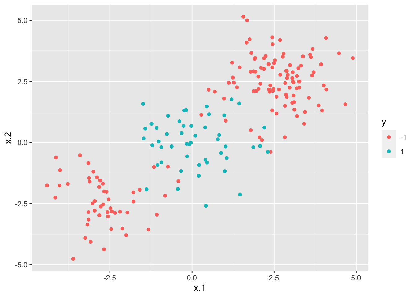
From the plot it results that the data can’t be separated by a linear decision boundary.
As usual, we split the data into a training and a test set. The first one, named simdata_tr, contains 70% of the observations. The latter is named simdata_te.
set.seed(4,sample.kind = "Rejection")
index = sample(1:nrow(simdata),0.7*nrow(simdata))
simdata_tr = simdata[index,]
simdata_te = simdata[-index,]
7.1 Adaboost
By using the adaboost function (see ?adaboost) contained in the fastAdaboost package, we train the Adaboost algorithm for predicting the category of the response variable y. We start by using a number of iterations (nIter) equal to 20 (this corresponds to the term \(M\) in the theory slides #12).
## adaboost(formula = y ~ ., data = simdata_tr, nIter = 20)
## y ~ .
## Dependent Variable: y
## No of trees:20
## The weights of the trees are:1.401681.2278050.86983751.0010750.83209920.99527540.70318890.96153970.66162650.71430790.70110170.76249940.80928390.73319420.90942961.0593050.59021690.54642260.62977050.4121731
Given the estimated model we estimate the predicted category for the test observations and then compute the accuracy of the algorithm.
Note that ada1 is a list containing several objects
## [1] "formula" "votes" "class" "prob" "error"For obtaining the confusion matrix and computing accuracy we will need the object named class containing the predicted categories.
##
##      -1  1
##   -1 44  2
## 1 3 11## [1] 0.9166667We wonder if it is possible to obtain a higher accuracy by changing the values of the tuning parameter nIter. Similarly to what is described in Section 6.3, we use a for loop to run the Adaboost algorithm by using different values for the number of iterations. In particular we use the regular sequence of values from 1 to 5000 with step (the increment) equal to 5. For each step of the for loop we save the accuracy.
out = data.frame(iter=seq(1,1000,by=5))
for(i in 1:nrow(out)){
  fastadaboost <- adaboost(y ~ .,
                           data = simdata_tr,
                           nIter = i)
  pred_fastadaboost <- predict(fastadaboost,newdata=simdata_te)
  out$acc[i] = mean(pred_fastadaboost$class==simdata_te$y)
}
head(out)
## iter acc
## 1 1 0.9333333
## 2 6 0.9333333
## 3 11 0.9333333
## 4 16 0.9333333
## 5 21 0.8833333
## 6 26 0.9000000We analyse the accuracy by means of a plot with the number of iteration on the x-axis and the accuracy on the y-axis.
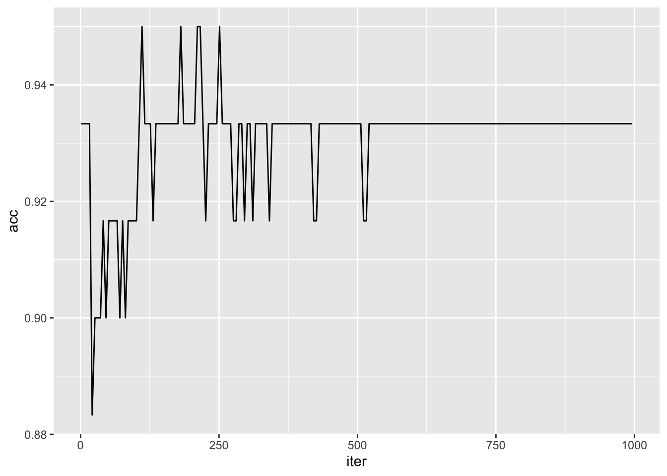 It seems that starting from the value 521 the accuracy and equal to 0.93. We thus estimate a new model and compute the prediction for this case:
7.2 LDA and QDA
We compare, by means of accuracy, the Adaboost algorithm with linear and quadratic discriminant analysis (LDA and QDA).
library(MASS)
#LDA
lda_simdata = lda(y ~ .,
                  data = simdata_tr)
pred_lda <- predict(lda_simdata,
                    newdata=simdata_te)
table(pred_lda$class, simdata_te$y)
##
## -1 1
## -1 47 13
## 1 0 0## [1] 0.7833333#QDA
qda_simdata = qda(y ~ .,
data = simdata_tr)
pred_qda <- predict(qda_simdata,
newdata=simdata_te)
table(pred_qda$class, simdata_te$y)##
## -1 1
## -1 47 6
## 1 0 7## [1] 0.9We can conclude that …..
7.3 SVM
We use the same data (simdata_tr and simdata_te) to implement SVM by using the function svm contained in the e1071 library (see ?svm). In particular, given the structure of the data a linear kernel won’t be taken into account; we will use instead a radial kernel.
We start by implement SVM with a radial kernel with \(\gamma=1\) and cost parameter \(C=1\).
##
## Call:
## svm(formula = y ~ ., data = simdata_tr, kernel = "radial", cost = 1,
##     gamma = 1)
##
##
## Parameters:
##    SVM-Type:  C-classification
##  SVM-Kernel:  radial
##        cost:  1
##
## Number of Support Vectors:  32
From the output we see that there are 32 training observations classified as support vectors. We can now use the function plot.svm to represent graphically the output (see ?plot.svm).
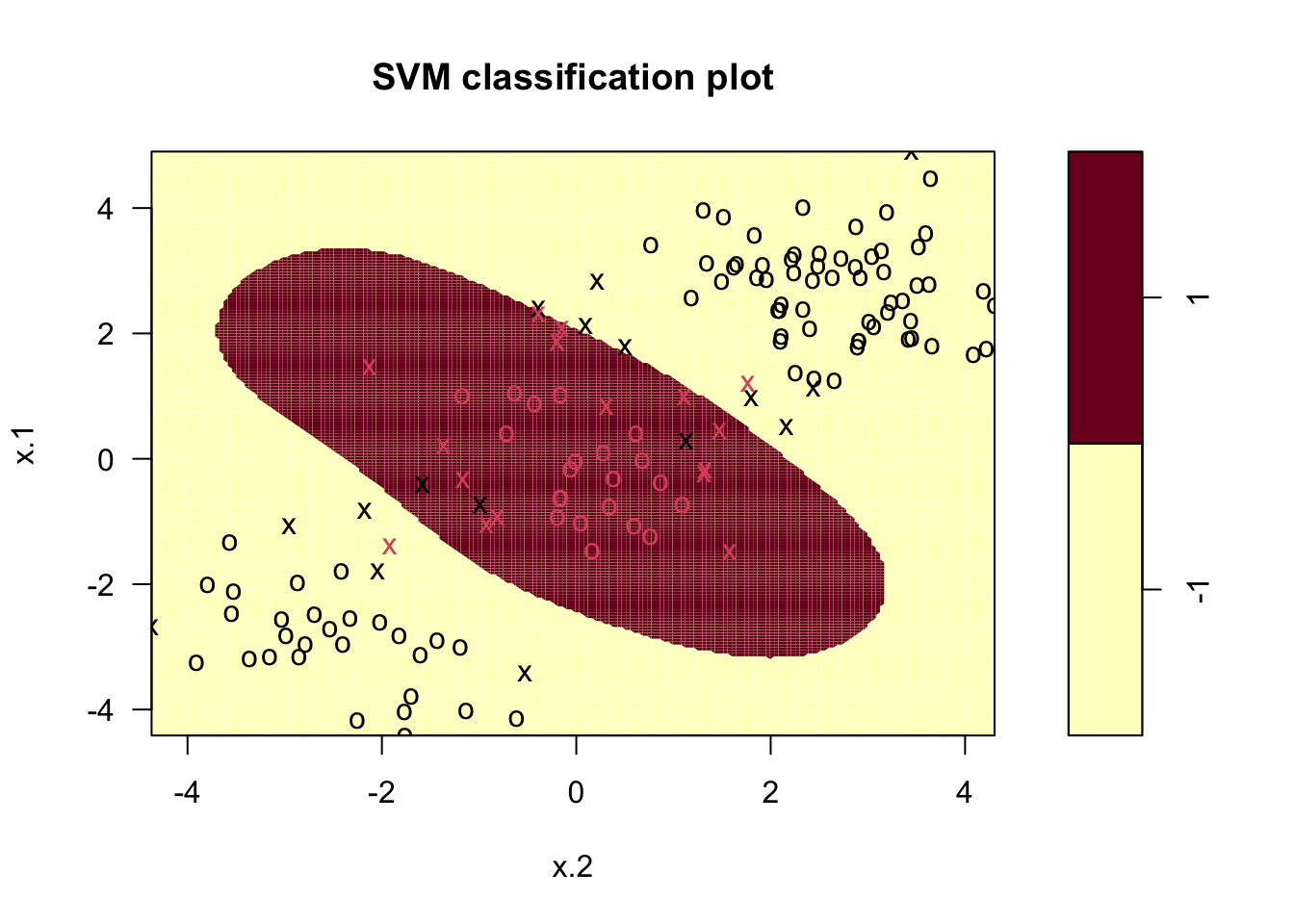 In the figure we see the training observations represented by different colors: red symbols belong to the category +1, while black symbols to the category -1. Crosses (instead of circles) are used to denote the support vectors. Finally the background color represents the predicted category: the red area defines the values of the regressors for which the prediction of
 y is equal to +1. Elsewhere (in the yellow area) the prediction will be given by category -1. The option grid of the plot function improves the resolution of the prediction areas (the higher the value, the higher the resolution).
As usual, we compute predictions and then the accuracy.
#predictions
pred_svm1 = predict(svm1, newdata=simdata_te)
#svm1 is a vector
#matrix
table(pred_svm1, simdata_te$y)
##
## pred_svm1 -1 1
## -1 45 2
## 1 2 11## [1] 0.9333333Let’s now change the value of \(\gamma\) to 2 (\(\gamma >0\)) and keep \(C=1\). How does the accuracy change?
svm2 = svm(y~.,
           data = simdata_tr,
           kernel = "radial",
           cost = 1,
           gamma = 2)
#predictions
pred_svm2 = predict(svm2, newdata=simdata_te)
#svm1 is a vector
#matrix
table(pred_svm2, simdata_te$y)
##
## pred_svm2 -1 1
## -1 45 3
## 1 2 10## [1] 0.9166667By changing the value of \(\gamma\) the accuracy decreases slightly.
Let’s now consider different values of \(C\) and \(\gamma\) and see which is the best combination in terms of cross-validation accuracy. In this case, instead of proceeding with a for loop as described for Adaboost, we will use the function tune implemented in the e1071 library (given that we use CV we set the seed equal to 1) . In particular, we consider for \(C\) the values cost=c(0.1,1,10,100,1000) and for \(\gamma\) the integers from 1 to 10 (1:10 or seq(1,10)). This will give rise to \(10 \times 5 = 50\) combinations of hyperparameters.
#?tune
set.seed(1,sample.kind = "Rejection")
tune.svm = tune(svm, #function to run iteratively
                y ~ .,
                data = simdata_tr,
                kernel = "radial",
                ranges = list(cost = c(0.1,1,10,100,1000),
                              gamma = 1:10))
By typing
##
## Parameter tuning of 'svm':
##
## - sampling method: 10-fold cross validation
##
## - best parameters:
##  cost gamma
##   0.1     1
##
## - best performance: 0.05714286
##
## - Detailed performance results:
##     cost gamma      error dispersion
## 1  1e-01     1 0.05714286 0.05634362
## 2  1e+00     1 0.06428571 0.07103064
## 3  1e+01     1 0.08571429 0.06563833
## 4  1e+02     1 0.09285714 0.06776309
## 5  1e+03     1 0.07142857 0.05832118
## 6  1e-01     2 0.08571429 0.06563833
## 7  1e+00     2 0.07142857 0.06734350
## 8  1e+01     2 0.08571429 0.05634362
## 9  1e+02     2 0.08571429 0.06563833
## 10 1e+03     2 0.10000000 0.07678341
## 11 1e-01     3 0.11428571 0.09035079
## 12 1e+00     3 0.07142857 0.06734350
## 13 1e+01     3 0.07857143 0.05270463
## 14 1e+02     3 0.07857143 0.06254250
## 15 1e+03     3 0.10000000 0.07678341
## 16 1e-01     4 0.15000000 0.09190600
## 17 1e+00     4 0.07857143 0.06254250
## 18 1e+01     4 0.07857143 0.05270463
## 19 1e+02     4 0.08571429 0.07377111
## 20 1e+03     4 0.10714286 0.10780220
## 21 1e-01     5 0.16428571 0.09553525
## 22 1e+00     5 0.08571429 0.08109232
## 23 1e+01     5 0.10000000 0.06023386
## 24 1e+02     5 0.09285714 0.08940468
## 25 1e+03     5 0.10000000 0.09642122
## 26 1e-01     6 0.20714286 0.10350983
## 27 1e+00     6 0.07857143 0.06254250
## 28 1e+01     6 0.10000000 0.06023386
## 29 1e+02     6 0.10000000 0.09642122
## 30 1e+03     6 0.10714286 0.09066397
## 31 1e-01     7 0.25000000 0.08417938
## 32 1e+00     7 0.09285714 0.06776309
## 33 1e+01     7 0.09285714 0.06776309
## 34 1e+02     7 0.10714286 0.09066397
## 35 1e+03     7 0.10714286 0.09066397
## 36 1e-01     8 0.26428571 0.10129546
## 37 1e+00     8 0.10000000 0.06900656
## 38 1e+01     8 0.10000000 0.07678341
## 39 1e+02     8 0.10714286 0.09066397
## 40 1e+03     8 0.10714286 0.09066397
## 41 1e-01     9 0.26428571 0.10129546
## 42 1e+00     9 0.10000000 0.06900656
## 43 1e+01     9 0.10000000 0.07678341
## 44 1e+02     9 0.10714286 0.09066397
## 45 1e+03     9 0.10714286 0.09066397
## 46 1e-01    10 0.26428571 0.10129546
## 47 1e+00    10 0.10714286 0.06941609
## 48 1e+01    10 0.10714286 0.08417938
## 49 1e+02    10 0.11428571 0.09642122
## 50 1e+03    10 0.11428571 0.09642122
we obtain a data frame with 50 rows (one for each hyperparameter combination). We are interested in the third column (error) giving us the cross-validation error for a specific value of cost and gamma. In particular, we look for the value of \(C\) and \(\gamma\) for which error is lowest. This information is provided automatically in the ouput of tune. In fact the object tune.svm (it’s a list) contains the following objects:
## [1] "best.parameters"  "best.performance" "method"           "nparcomb"
## [5] "train.ind"        "sampling"         "performances"     "best.model"
By using the $ we can extract the best combination of parameters ($best.parameters), the corresponding cv error ($best.performance) and the corresponding estimate svm model ($best.model):
##   cost gamma
## 1 0.1 1## [1] 0.05714286##
## Call:
## best.tune(method = svm, train.x = y ~ ., data = simdata_tr, ranges = list(cost = c(0.1,
## 1, 10, 100, 1000), gamma = 1:10), kernel = "radial")
##
##
## Parameters:
## SVM-Type: C-classification
## SVM-Kernel: radial
## cost: 0.1
##
## Number of Support Vectors: 72If you are interest in computing class predictions for the test observation given the best hyperparameter setting, you could use the object tune.svm$best.model directly in the predict function.
Here instead we will take another approach in view of the computation of the ROC curve. Besides class predictions we also need probabilities which in the case of svm is a transformation of the decision values (the latter is the computed values of the hyperplane equation). To obtain this additional information we will use the options decision.values = T,probability = T in the svm and predict functions (run with the best parameter setting).
svm2 = svm(y~.,
           data = simdata_tr,
           kernel = "radial",
           cost = as.numeric(tune.svm$best.parameters[1]),
           gamma = tune.svm$best.parameters[2],
           decision.values = T,
           probability = T)
svm2
##
## Call:
## svm(formula = y ~ ., data = simdata_tr, kernel = "radial", cost = as.numeric(tune.svm$best.parameters[1]),
## gamma = tune.svm$best.parameters[2], decision.values = T, probability = T)
##
##
## Parameters:
## SVM-Type: C-classification
## SVM-Kernel: radial
## cost: 0.1
##
## Number of Support Vectors: 72# compute predictions + decision.values + probabilities for the test set
pred_svm2 = predict(svm2,
newdata = simdata_te,
decision.values = T,
probability = T)
# accuracy
mean(pred_svm2 == simdata_te$y)## [1] 0.9By typing pred_svm2 or attributes(pred_svm2) we see that the object pred_svm2 contains more information than just the predicted categories. We are in particular interested in the attribute called "probabilities" which can be extracted as follows:
We are now able to compute and plot the ROC curve as described in Section 3.7:
## Setting levels: control = -1, case = 1## Setting direction: controls > cases## Setting levels: control = -1, case = 1
## Setting direction: controls > cases## Setting levels: control = -1, case = 1
## Setting direction: controls > cases## Setting levels: control = -1, case = 1
## Setting direction: controls > cases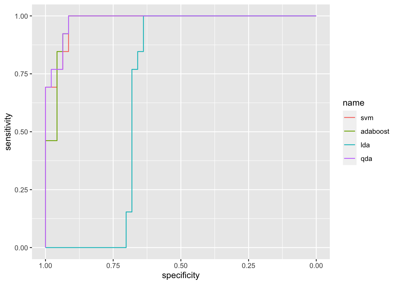
## Area under the curve: 0.9787## Area under the curve: 0.9722## Area under the curve: 0.6759## Area under the curve: 0.9827.4 SVM with more than 2 categories and more than 2 regressors
We consider now the Glass dataset contained in the mlbench library (see ?Glass). We start by exploring the data where Type is the response variale.
## Rows: 214
## Columns: 10
## $ RI   <dbl> 1.52101, 1.51761, 1.51618, 1.51766, 1.51742, 1.51596, 1.51743, 1.…
## $ Na   <dbl> 13.64, 13.89, 13.53, 13.21, 13.27, 12.79, 13.30, 13.15, 14.04, 13…
## $ Mg   <dbl> 4.49, 3.60, 3.55, 3.69, 3.62, 3.61, 3.60, 3.61, 3.58, 3.60, 3.46,…
## $ Al   <dbl> 1.10, 1.36, 1.54, 1.29, 1.24, 1.62, 1.14, 1.05, 1.37, 1.36, 1.56,…
## $ Si   <dbl> 71.78, 72.73, 72.99, 72.61, 73.08, 72.97, 73.09, 73.24, 72.08, 72…
## $ K    <dbl> 0.06, 0.48, 0.39, 0.57, 0.55, 0.64, 0.58, 0.57, 0.56, 0.57, 0.67,…
## $ Ca   <dbl> 8.75, 7.83, 7.78, 8.22, 8.07, 8.07, 8.17, 8.24, 8.30, 8.40, 8.09,…
## $ Ba   <dbl> 0, 0, 0, 0, 0, 0, 0, 0, 0, 0, 0, 0, 0, 0, 0, 0, 0, 0, 0, 0, 0, 0,…
## $ Fe   <dbl> 0.00, 0.00, 0.00, 0.00, 0.00, 0.26, 0.00, 0.00, 0.00, 0.11, 0.24,…
## $ Type <fct> 1, 1, 1, 1, 1, 1, 1, 1, 1, 1, 1, 1, 1, 1, 1, 1, 1, 1, 1, 1, 1, 1,…
We see that the response variable is characterized by 6 categories:
##
##  1  2  3  5  6  7
## 70 76 17 13  9 29
We proceed with some descriptive plotting:
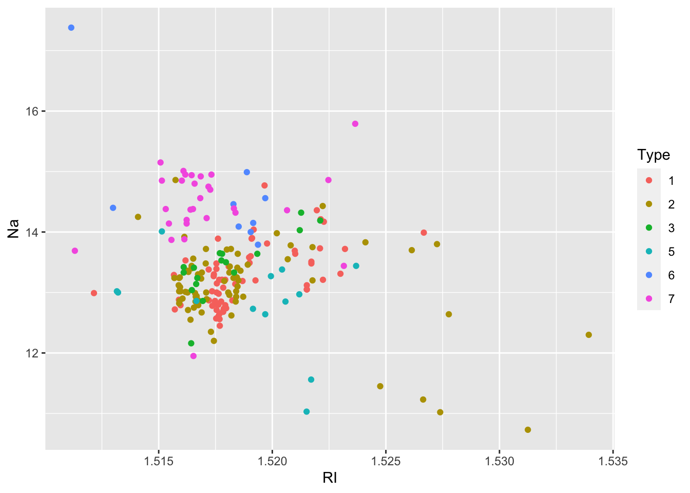
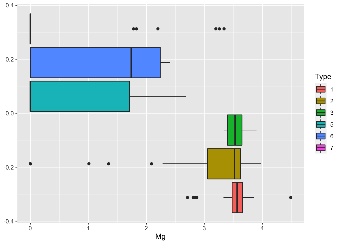
We then create as usual the training (70%) and test data set.
set.seed(44,sample.kind = "Rejection")
tr_index = sample(1:nrow(Glass), nrow(Glass)*0.7)
Glass_tr = Glass[tr_index,]
Glass_te = Glass[-tr_index,]
Finally, we implement SVM. Note that the function svm uses the one-against-one approach. We consider in this case a polynomial kernel of degree \(d\) 1 and a value of \(C=1\). We then compute predictions and accuracy.
svm.fit = svm(Type ~ .,
              data = Glass_tr,
              kernel = "polynomial",
              cost = 1,
              degree = 1)
svm.pred = predict(svm.fit,
                   Glass_te)

table(svm.pred, Glass_te$Type)
##
## svm.pred 1 2 3 5 6 7
## 1 21 11 2 0 0 0
## 2 2 12 1 2 0 0
## 3 0 0 0 0 0 0
## 5 0 1 0 0 0 0
## 6 0 2 0 0 0 0
## 7 0 1 0 3 0 7## [1] 0.6153846To tune the hyperparameters we consider different values of \(C\) (cost=c(0.1,1,10,100,1000)) and of the degree of the polynomial(1:5) and then compute the accuracy for each combination of hyperparameters.
set.seed(1,sample.kind = "Rejection")
tune.out=tune(svm,
              Type ~ .,
              data = Glass_tr,
              kernel="polynomial",
              ranges=list(cost=c(0.1,1,10,100,1000),
                          degree=1:5))
summary(tune.out)
##
## Parameter tuning of 'svm':
##
## - sampling method: 10-fold cross validation
##
## - best parameters:
## cost degree
## 1000 3
##
## - best performance: 0.3142857
##
## - Detailed performance results:
## cost degree error dispersion
## 1 1e-01 1 0.5838095 0.07566619
## 2 1e+00 1 0.3952381 0.11306669
## 3 1e+01 1 0.3542857 0.10697989
## 4 1e+02 1 0.3209524 0.11070675
## 5 1e+03 1 0.3347619 0.10228062
## 6 1e-01 2 0.5966667 0.07445274
## 7 1e+00 2 0.5095238 0.09735737
## 8 1e+01 2 0.3747619 0.18767853
## 9 1e+02 2 0.3147619 0.13592437
## 10 1e+03 2 0.3480952 0.17874524
## 11 1e-01 3 0.6104762 0.07005019
## 12 1e+00 3 0.5300000 0.09993825
## 13 1e+01 3 0.3614286 0.12051895
## 14 1e+02 3 0.3547619 0.15259988
## 15 1e+03 3 0.3142857 0.12832624
## 16 1e-01 4 0.5761905 0.10021393
## 17 1e+00 4 0.5566667 0.10189561
## 18 1e+01 4 0.4890476 0.10079178
## 19 1e+02 4 0.3619048 0.13997084
## 20 1e+03 4 0.3347619 0.12801270
## 21 1e-01 5 0.5685714 0.13333711
## 22 1e+00 5 0.5566667 0.09692813
## 23 1e+01 5 0.5100000 0.11764143
## 24 1e+02 5 0.4561905 0.09706709
## 25 1e+03 5 0.3890476 0.13903258## cost degree
## 15 1000 3# prediction (based on the one-versus-one approach)
svm.pred.best = predict(tune.out$best.model,
newdata=Glass_te)
table(svm.pred.best, Glass_te$Type)##
## svm.pred.best 1 2 3 5 6 7
## 1 19 4 2 1 0 0
## 2 2 17 0 3 0 1
## 3 2 2 1 0 0 0
## 5 0 1 0 0 0 0
## 6 0 2 0 0 0 0
## 7 0 1 0 1 0 6## [1] 0.6615385Note that in this case the confusion matrix is not a 2 by 2 matrix, but it’s dimension is given by the number of categories of the response variable.
7.5 Exercises Lab 6
The RMarkdown file Lab6_home_exercises_empty.Rmd contains the exercise for Lab 6. Write your solutions in the RMarkdown file and produce the final html file containing your code, your comments and all the outputs.