Chapter 3 R Lab 2 - 15/04/2021
In this lecture we will learn how to implement the logistic regression model, the linear and the quadratic discriminant analysis (LDA and QDA).
The following packages are required: MASS, pROC and tidyverse.
##
## Attaching package: 'MASS'
## The following object is masked from 'package:dplyr':
##
## select## Type 'citation("pROC")' for a citation.##
## Attaching package: 'pROC'## The following objects are masked from 'package:stats':
##
## cov, smooth, var3.1 Diabetes data
The data we use for this lab are from the Kaggle platform link. The objective of the analysis is to predict whether or not a patient has diabetes, based on certain diagnostic measurements.
The datasets consists of several predictor variables:
Pregnancies: Number of pregnanciesGlucose: Plasma glucose concentration a 2 hours in an oral glucose tolerance testBloodPressure: Diastolic blood pressure (mm Hg)SkinThickness: Triceps skin fold thickness (mm)Insulin: 2-Hour serum insulin (mu U/ml)BMI: Body mass index (weight in kg/(height in m)^2)DiabetesPedigreeFunction: Diabetes pedigree functionAge: Age (years)
The response variable is named Outcome and is a binary variable: 0 means that the patient does not have diabetes, while 1 means the patient does have diabetes.
We import the data
diabetes <- read.csv("~/Dropbox/UniBg/Didattica/Economia/2020-2021/MLFE_2021/RLabs/Lab2/diabetes.csv")
glimpse(diabetes)
## Rows: 768
## Columns: 9
## $ Pregnancies <int> 6, 1, 8, 1, 0, 5, 3, 10, 2, 8, 4, 10, 10, 1, …
## $ Glucose <int> 148, 85, 183, 89, 137, 116, 78, 115, 197, 125…
## $ BloodPressure <int> 72, 66, 64, 66, 40, 74, 50, 0, 70, 96, 92, 74…
## $ SkinThickness <int> 35, 29, 0, 23, 35, 0, 32, 0, 45, 0, 0, 0, 0, …
## $ Insulin <int> 0, 0, 0, 94, 168, 0, 88, 0, 543, 0, 0, 0, 0, …
## $ BMI <dbl> 33.6, 26.6, 23.3, 28.1, 43.1, 25.6, 31.0, 35.…
## $ DiabetesPedigreeFunction <dbl> 0.627, 0.351, 0.672, 0.167, 2.288, 0.201, 0.2…
## $ Age <int> 50, 31, 32, 21, 33, 30, 26, 29, 53, 54, 30, 3…
## $ Outcome <int> 1, 0, 1, 0, 1, 0, 1, 0, 1, 1, 0, 1, 0, 1, 1, …We transform this 0/1 integer variable into a factor with categories “No” and “Yes”:
##
## No Yes
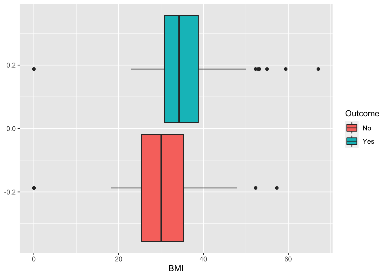
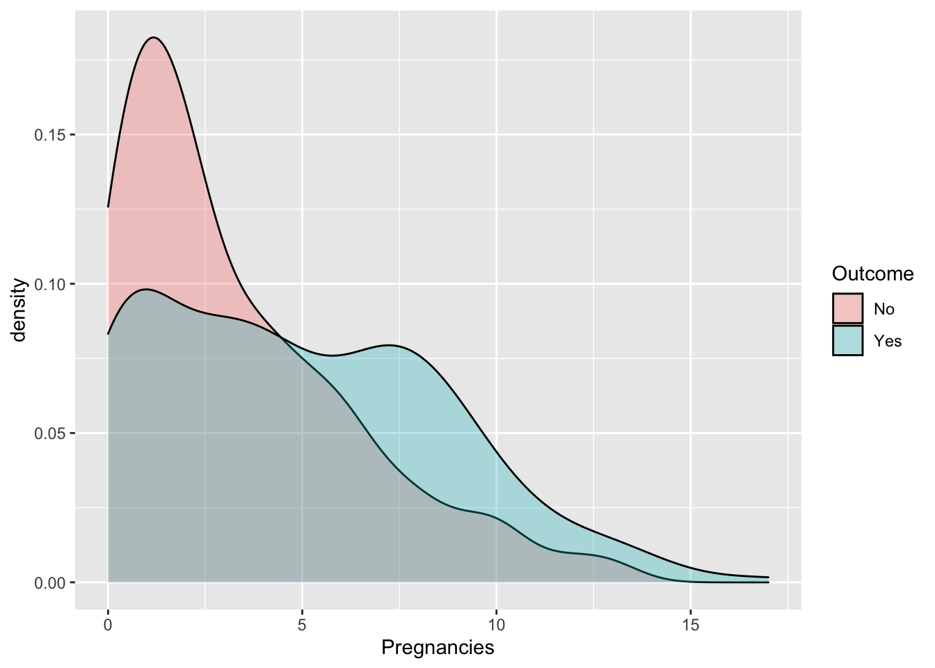
## 500 268Some exploratory analysis can be done to study the distribution of the regressors conditionally on the diabetes condition. We consider here, as an example, BMI or Pregnancies:
3.2 Definition of a function for computing performance indexes
For assessing the performance of a classifier we compare predicted categories with observed categories. This can be done by using the confusion matrix which is a 2x2 matrix reporting the joint distribution (with absolute frequencies) of predicted (by row) and observed (by column) categories.
| No (obs.) | Yes (obs.) | |||
|---|---|---|---|---|
| No (pred.) | TN | FN | ||
| Yes (pred.) | FP | TP | ||
| Total | N | P |
We consider in particular the following performance indexes:
- sensitivity (true positive rate): TP/P
- specificity (true negative rate): TN/N
- accuracy (rate of correctly classified observations): (TN+TP)/(N+P)
We define a function named perf_indexes which computes the above defined indexes. The function has only one argument which is a confusion 2x2 matrix named cm. It returns a vector with the 3 indexes.
3.3 A new method for creating the training and testing set
To create the training (70%) and test (30%) dataset we use a new approach different from the one introduced in Section 2.1.1.
We first create in the dataframe a new column that contains an unique ID for each observation (this will be used later). The ID is simply given by the row number of each observation and can be obtained by usinf the row_number function:
##   Pregnancies Glucose BloodPressure SkinThickness Insulin  BMI
## 1           6     148            72            35       0 33.6
## 2           1      85            66            29       0 26.6
## 3           8     183            64             0       0 23.3
## 4           1      89            66            23      94 28.1
## 5           0     137            40            35     168 43.1
## 6           5     116            74             0       0 25.6
##   DiabetesPedigreeFunction Age Outcome id
## 1                    0.627  50     Yes  1
## 2                    0.351  31      No  2
## 3                    0.672  32     Yes  3
## 4                    0.167  21      No  4
## 5                    2.288  33     Yes  5
## 6                    0.201  30      No  6
We are now ready to sample from the diabetes dataset 70% of the observations (rows) by using the slice_sample function:
##   Pregnancies Glucose BloodPressure SkinThickness Insulin  BMI
## 1           9     170            74            31       0 44.0
## 2           6      92            92             0       0 19.9
## 3           7     142            90            24     480 30.4
## 4          10     108            66             0       0 32.4
## 5           1      89            76            34      37 31.2
## 6           1     164            82            43      67 32.8
##   DiabetesPedigreeFunction Age Outcome  id
## 1                    0.403  43     Yes 762
## 2                    0.188  28      No  34
## 3                    0.128  43     Yes 696
## 4                    0.272  42     Yes 144
## 5                    0.192  23      No 113
## 6                    0.341  50      No 549
To get now the test set we use the anti_join function. As reported in the following fiugre
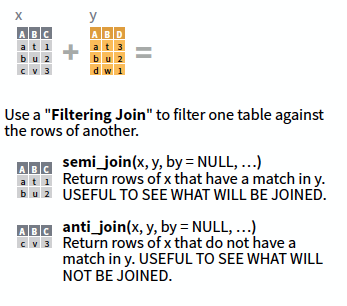
the anti_join function returns the rows of a first dataframe (for us diabetes) which are not cointained in a second dataframe (for us tr). For this operation it is necessary to specify an ID variable which is available in both the dataframes: it’s the ID variable that we have created before!
##   Pregnancies Glucose BloodPressure SkinThickness Insulin  BMI
## 1           2     197            70            45     543 30.5
## 2           8     125            96             0       0  0.0
## 3           4     110            92             0       0 37.6
## 4           1     189            60            23     846 30.1
## 5           1     115            70            30      96 34.6
## 6           7     147            76             0       0 39.4
##   DiabetesPedigreeFunction Age Outcome id
## 1                    0.158  53     Yes  9
## 2                    0.232  54     Yes 10
## 3                    0.191  30      No 11
## 4                    0.398  59     Yes 14
## 5                    0.529  32     Yes 20
## 6                    0.257  43     Yes 27
We now remove from tr and te the ID variable as it is not useful for the following analysis:
3.4 Logistic regression
For implementing the logistic regression the function glm (generalized linear model) is used. It requires the specification of the formula, of the dataframe containing the data and of the distribution (family) of the response variable (in this case binomial distribution given that we are working with a binary response):
##
## Call:
## glm(formula = Outcome ~ ., family = "binomial", data = tr)
##
## Deviance Residuals:
##     Min       1Q   Median       3Q      Max
## -2.5055  -0.7661  -0.4241   0.7973   2.7234
##
## Coefficients:
##                            Estimate Std. Error z value Pr(>|z|)
## (Intercept)              -8.2035808  0.8562214  -9.581  < 2e-16 ***
## Pregnancies               0.1193692  0.0381312   3.130  0.00175 **
## Glucose                   0.0317281  0.0041851   7.581 3.42e-14 ***
## BloodPressure            -0.0151853  0.0066067  -2.298  0.02153 *
## SkinThickness             0.0008759  0.0079027   0.111  0.91175
## Insulin                  -0.0011698  0.0010986  -1.065  0.28694
## BMI                       0.1032936  0.0185240   5.576 2.46e-08 ***
## DiabetesPedigreeFunction  0.8886256  0.3439073   2.584  0.00977 **
## Age                       0.0153383  0.0112087   1.368  0.17118
## ---
## Signif. codes:  0 '***' 0.001 '**' 0.01 '*' 0.05 '.' 0.1 ' ' 1
##
## (Dispersion parameter for binomial family taken to be 1)
##
##     Null deviance: 703.68  on 536  degrees of freedom
## Residual deviance: 519.01  on 528  degrees of freedom
## AIC: 537.01
##
## Number of Fisher Scoring iterations: 5
Note that the notation Outcome ~. means that all the covariates but Outcome are included as regressors (this avoids to write the formula in the standard way: Outcome ~ Pregnancies+Glucose+...).
The summary contains the parameter estimates and the corresponding p-values of the test checking \(H_0:\beta =0\) vs \(H_1: \beta\neq 0\). Consider for example the parameter of the Pregnancies variable which is positive (i.e. higher risk of diabetes) and equal to 0.1193692: this means that for a one-unit increase in the number of pregnancies, the log-odds increases by 0.1193692. For a simpler interpretation, in the odds scale, we can take the exponential transformation of the parameter:
## Pregnancies
##    1.126786
This means that this means that for a one-unit increase in the number of pregnancies, we expect a 12.68 increase in the diabetes odds (remember that the odds is strictly connected to the diabetes probability as it is defined as \(p/(1-p)\)).
We are now interested in computing predictions for the test observations given the estimated logistic model. They can be obtained by using the predict.glm function. It is important to specify that we are interested in the prediction on the outcome scale (otherwise we will get the predictions on the logit scale);
##          1          2          3          4          5          6
## 0.67493875 0.02398662 0.24613189 0.59857381 0.25929919 0.75019202
The object logreg_pred contains the conditional probability of having diabetes given the covariate vector. For example for the first test observation the diabetes probability is equal to logreg_pred[1]. In order to have a categorical prediction it is necessary to fix a threshold for the probability (default is 0.5) and transform correspondingly the probabilities:
##     1     2     3     4     5     6
## "Yes"  "No"  "No" "Yes"  "No" "Yes"
As expected, the predicted category for the first observation is “Yes”.
We are now ready to compute the confusion matrix
##
## logreg_pred_cat  No Yes
##             No  140  27
##             Yes  18  46
and the performance index by using the function we defined in Section 3.2
##      sens      spec       acc
## 0.6301370 0.8860759 0.8051948
3.5 Linear and quadratic discriminant analysis
To run LDA we use the lda function of the MASS package. Similarly, to logistic regression we have to specify the formula and the data:
## Call:
## lda(Outcome ~ ., data = tr)
##
## Prior probabilities of groups:
##        No       Yes
## 0.6368715 0.3631285
##
## Group means:
##     Pregnancies  Glucose BloodPressure SkinThickness  Insulin      BMI
## No     3.304094 110.0409      68.45322      19.58187 66.75146 30.21228
## Yes    4.846154 140.4564      71.47179      22.69231 94.42564 35.15077
##     DiabetesPedigreeFunction      Age
## No                 0.4269415 31.16667
## Yes                0.5597333 36.84615
##
## Coefficients of linear discriminants:
##                                    LD1
## Pregnancies               0.0929390001
## Glucose                   0.0247988603
## BloodPressure            -0.0129578404
## SkinThickness             0.0012477089
## Insulin                  -0.0008439518
## BMI                       0.0698160977
## DiabetesPedigreeFunction  0.6347798644
## Age                       0.0125305304
The output reports the prior probabilities for the two categories and the conditional means of all the covariates.
We go straight to the calculation of the predictions:
## [1] "class" "posterior" "x"Note that the object lda_pred is a list containing 3 objects including the vector of posterior probabilities (posterior) and the vector of predicted categories (`class):
##          No        Yes
## 1 0.2871729 0.71282712
## 2 0.9683246 0.03167541
## 3 0.7805098 0.21949024
## 4 0.3587903 0.64120969
## 5 0.7525345 0.24746553
## 6 0.2584910 0.74150900## [1] Yes No No Yes No Yes
## Levels: No YesTo compute the confusion matrix we will use the vector lda_pred$class:
##
##        No Yes
##   No  143  28
## Yes 15 45## sens spec acc
## 0.6164384 0.9050633 0.8138528For the quadratic discriminant analysis everything is very similar except the use of the function qda instead of lda:
## Call:
## qda(Outcome ~ ., data = tr)
##
## Prior probabilities of groups:
##        No       Yes
## 0.6368715 0.3631285
##
## Group means:
##     Pregnancies  Glucose BloodPressure SkinThickness  Insulin      BMI
## No     3.304094 110.0409      68.45322      19.58187 66.75146 30.21228
## Yes    4.846154 140.4564      71.47179      22.69231 94.42564 35.15077
##     DiabetesPedigreeFunction      Age
## No                 0.4269415 31.16667
## Yes 0.5597333 36.84615## [1] "class" "posterior"## [1] Yes No No Yes No Yes
## Levels: No Yes## No Yes
## 1 1.132643e-04 0.99988674
## 2 9.828051e-01 0.01719485
## 3 7.994316e-01 0.20056835
## 4 3.567559e-10 1.00000000
## 5 8.683338e-01 0.13166621
## 6 3.345753e-01 0.66542467## sens spec acc
## 0.6301370 0.8417722 0.77489183.6 Classifiers comparison in terms of performance indexes
By comparing the 3 classifiers with respect to accuracy, sensitivity and specificity
##      sens      spec       acc
## 0.6301370 0.8860759 0.8051948## sens spec acc
## 0.6164384 0.9050633 0.8138528## sens spec acc
## 0.6301370 0.8417722 0.7748918we see that the logistic regression and LDA perform very similarly. In particular, LDA has the highest specificity but the lowest sensitivity. In terms of accuracy it has the best performance. The QDA instead is the poorest between the three tested methods.
3.7 Construction and plotting of the ROC curve
To obtain the ROC curve we use the function roc contained in the pROC package. It is necessary to specify as arguments the vector of observed categories (response) and the vector of the probabilities for the “Yes” category (predictor).
## Setting levels: control = No, case = Yes## Setting direction: controls < casesGiven the ROC curve it is possible to plot it and to compute the area under the curve (auc):
## Area under the curve: 0.8407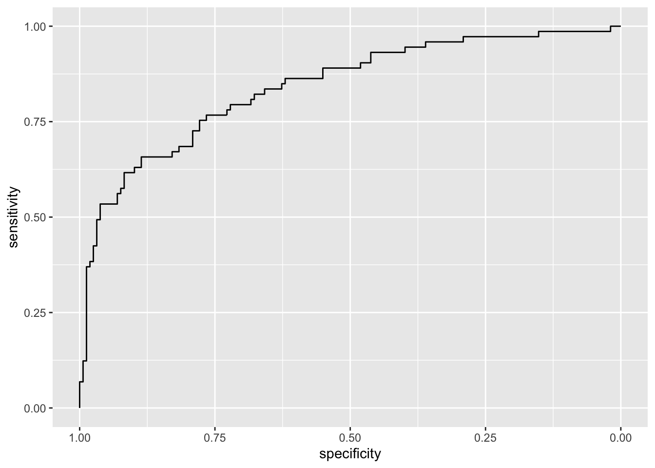 Note that the plot uses specificity on the x-axis (which goes from 1 on the left to zero on the right) and sensitivity on the y-axis.
We now compute all the ROC curves and plot them together using the ggroc function:
roc_lda = roc(response = te$Outcome,
              predictor = lda_pred$posterior[,2]) #the second col. contains the probabilities for the yes category
## Setting levels: control = No, case = Yes## Setting direction: controls < cases## Setting levels: control = No, case = Yes
## Setting direction: controls < cases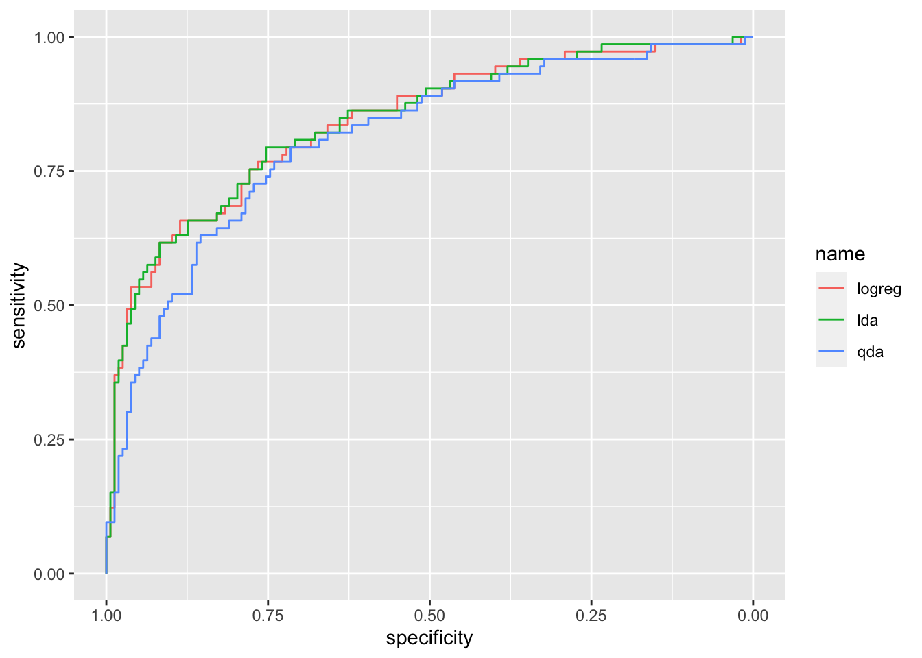
It can be observed that the ROC curve lies below the other two curves meaning that QDA performs worse. Let’s compute the auc for the three methods:
## Area under the curve: 0.8407## Area under the curve: 0.8419## Area under the curve: 0.8111LDA shows the highest auc (even if very similar to the logistic regression auc). All in all we can conclude that LDA is the best classifier.
3.8 Exercises Lab 2
3.8.1 Exercise 1
The data contained in the files titanic_tr.csv (for training) and titanic_te.csv (and testing) are about the Titanic disaster (the files are available in the e-learning). In particular the following variables are available:
pclass: ticket class (1 = 1st, 2 = 2nd, 3 = 3rd)survived: survival (0 = No, 1 = Yes)nameof the passengersexagein yearssibsp: number of siblings / spouses aboard the Titanicparchnumber of parents / children aboard the Titanicticket: ticket numberfare: passenger farecabin: cabin numberembarked: port of Embarkation (C = Cherbourg, Q = Queenstown, S = Southampton)
Import the data in R and explore them. Note that the response variable is survived which is classified as a int 0/1 variable in the dataframe. Transform it in a factor type object using the factor function with categories “No” and “Yes”.
Convert
pclass(ticket class) to factor (1 = “1st”, 2 = “2nd”, 3 = “3rd”) for both the training and test data set. Plotsurvivedas a function ofpclass. In which class do you observe the highest proportion of survivors?Check how many missing values we have in the variables
ageandfareseparately for training and test data.
- Separately for the training and test data, substitute the missing values with the average of
ageandfare. Note that for computing the mean when you have missing values you have to runmean(...,na.rm=T). After this, check that you don’t have any other missing values.
Consider the training data and
survivedas response variable. Compute the percentage of survived people. Moreover, represent graphically the relationship betweenageandsurvived. Comment the plot.Consider the training data set, estimate a logistic model for
survivedconsideringageas the only predictor (mod1). Provide the model summary.
Comment the
agecoefficient.Compute manually (without using
predict) by means of the formula of the logistic function the probability of surviving for a person of 50 years old. Remember that estimated coefficients can be retrieved bymod1$coefficients. Repeat the same for a person of 20 years old. Finally compute the odds and the odds-ratio.Compute the probability of surviving for all the people in the test data set (use
predict).Plot the estimated probabilities as a function of age (impose that the probability axis is between 0 and 1). Use for each point a color corresponding to the
survivedoutcome. Moreover, include in the plot an horizontal line corresponding to the probability threshold (0.5) and the corresponding age threshold (age boundary between categories). Comment the plot.Compute the confusion matrix for
mod1. Moreover, compute the test classification error rate.
- Consider the training data set, estimate a logistic model for
survivedconsideringpclassas predictor (mod2). Note thatpclassis a categorical variable with 3 categories and will be included in the model as a dummy variable with 3-1 categories (one category is the baseline). Provide the model summary and comment the coefficients. The following functioncontrastshelps you in understanding which is the baseline category:
contrasts(tr$pclass)
# on the rows you have the categories
# on the column the 2 dummy variables that will be included in the model (for the 2nd and 3rd category)
#the baseline is the category 1st
#in the model 2 coefficients will be estimated for category 2nd and 3rd
For more information about the management of dummy variables in R please read this short note available here. It refers to a linear regression model but it generalizes to any model.
Compute (manually or by using
predict) the probability of surviving for a person with a 1st class ticket. Repeat also for the other 2 classes. Compare the three predicted probabilities with the corresponding surviving proportion computed for each class.Estimate the probability of surviving (and the corresponding categories) for all the observations in the test data set (using
predict). Then compute the test overall classification error rate and compare it with the one obtained formod1.
For the training observations represent graphically
fare(amount paid for the ticket) as a function ofpclass. Moreover, compute the average and medianfareamount separately for each class.Consider the training data set, estimate a logistic model for
survivedconsideringageandfareas predictors (mod3). Provide the model summary.
Comment the coefficient of
fare.Using
mod3compute the predicted probability of surviving for all the test observations and the corresponding categories.Plot
fare(y-axis) as a function ofageusing the predicted categories to color the points. Moreover, include in the plot the linear boundary (it’s the solution of $_0+_1 X_1+_2X_2=0) which separates the two groups.Given the previous plot, what’s the prediction for a 40 years old individual who paid 200 dollars ?
Compute the test error rate for
mod3and compare it with the other models.
- Consider the training data set, estimate a logistic model for
survivedconsideringage,fareandpclassas predictors (mod4). Provide the model summary. Comparemod4with the others by using the test classification error. Which is the best model?
3.8.2 Exercise 2
We will use some simulated data available from the mlbench library (don’t forget to install it) with \(p=2\) regressors and a binary response variable. Use the following code to generate the data and create the data frame.
library(mlbench)

?mlbench.circle
set.seed(3333,sample.kind="Rejection")
data = mlbench.circle(1000) #simulate 1000 data
datadf = data.frame(data$x,
                    Y=factor(data$classes,labels=c("No","Yes")))
head(datadf)
## X1 X2 Y
## 1 0.4705415 -0.52006500 No
## 2 -0.1253492 0.20921556 No
## 3 -0.4381452 0.52445868 No
## 4 0.5877131 -0.86523067 Yes
## 5 0.1631693 -0.01084204 No
## 6 -0.6190528 -0.98775598 YesPlot the data (use the response variable to color the points).
Split the dataset in two parts: 80% of the observations are used for training and 20% for testing. The split is random (use as seed for random number generation the number 456).
Estimate a logistic regression model using
X1andX2as regressors. Provide the model summary.Comment the model coefficients.
Plot the training data and add to the plot the linear decision boundary (see the slides for the formula) defined by the logistic model. Do you think that the model is working well?
Compute the predictions using the test observations. Provide the confusion matrix (use 0.5 as probability threshold) and the overall classification error rate.
Define a function named
classification_perfwhich computes the overall classification error rate, the sensitivity and the specificity for a 2x2 confusion matrix which has in the rows the predicted categories and in the columns the observed categories.Use the
classification_perffunction for the logistic regression model output. Comment about the performance of the logistic regression model.Consider now a very simple classifier (null classifier) which uses as prediction for all the test observations the majority class observed in the training dataset (regardless of the values of the predictors). Compute the overall error rate for the null classifier. Does it perform better than the logistic regression model?
Use linear discriminant analysis to classify your data. Compute the predictions using the test observations and provide the confusion matrix together with performance indexes. Comment the results.
- [Advanced and optional] Using a grid of values for
X1andX2together with theouterfunction, plot the decision boundary together with the training data. Add to the plot also the boundary estimated with the logistic model.
- [Advanced and optional] Using a grid of values for
Use quadratic discriminant analysis to classify your data. Compute the predictions using the test observations and provide the confusion matrix together with performance indexes. Comment the results.
- [Advanced and optional] Using a grid of values for
X1andX2together with theouterfunction, plot the decision boundary together with the training data. Add to the plot also the boundary estimated with the logistic model.
- [Advanced and optional] Using a grid of values for
Compute and plot the ROC curves for all the estimated models (lr, lda, qda). For which model do we obtain the highest area under the ROC curve?
3.8.3 Exercise 3
We will use some simulated data available from the mlbench library with \(p=2\) regressors and a response variable with 4 categories. Use the following code to generate the data.
library(mlbench)

?mlbench.smiley
set.seed(3333,sample.kind="Rejection")
data = mlbench.smiley(1000) #simulate 1000 data
datadf = data.frame(data$x, factor(data$classes))
head(datadf)
## x4 V2 factor.data.classes.
## 1 -0.7371167 0.9282289 1
## 2 -0.8580089 1.0668791 1
## 3 -0.7794051 1.0191270 1
## 4 -0.9232296 0.9328375 1
## 5 -0.7723922 0.9318714 1
## 6 -0.9142181 0.8255049 1## x1 x2 y
## 1 -0.7371167 0.9282289 1
## 2 -0.8580089 1.0668791 1
## 3 -0.7794051 1.0191270 1
## 4 -0.9232296 0.9328375 1
## 5 -0.7723922 0.9318714 1
## 6 -0.9142181 0.8255049 1##
## 1 2 3 4
## 167 167 250 416Plot the data (use the response variable to color the points).
Split the dataset in two parts: 70% of the observations are used for training and 20% for testing. The split is random (use as seed for random number generation the number 456).
Consider linear and quadratic discriminant analysis for your data. Compare the two classifiers.
Use the KNN method to classify your data. Choose the best value of \(k\) among a sequence of values between 1 and 100 (with step equal to 5). To tune the hyperparameter \(k\) split the training dataset into two sets: one for training (70%) and one for validation (30%). Use a seed equal to 4.
Which model (between lda, qda and knn) do you prefer? Explain why.