Chapter 5 R Lab 4 - 06/05/2021
In this lecture we will learn how to implement classification trees and their extensions (bagging and random forest).
The following packages are required: rpart, rpart.plot, randomForest and tidyverse and pROC.
library(rpart) #for CART
library(rpart.plot) #for plotting CART
library(randomForest) #for bagging+RF
library(tidyverse)
library(pROC)
5.1 Credit data and classification tree
The file credit.csv contains information about the default status (yes or no) of more than 500 individuals. Together with the response variable named default, 4 regressors are available. Here below the preview of the data:
credit = read.csv("~/Dropbox/UniBg/Didattica/Economia/2020-2021/MLFE_2021/RLabs/Lab4/credit.csv")
glimpse(credit)
## Rows: 522
## Columns: 5
## $ months_loan_duration <int> 48, 42, 24, 36, 30, 12, 48, 12, 24, 15, 24, 24, 6…
## $ percent_of_income <int> 2, 2, 3, 2, 4, 3, 3, 1, 4, 2, 4, 4, 2, 1, 3, 1, 3…
## $ years_at_residence <int> 2, 4, 4, 2, 2, 1, 4, 1, 4, 4, 2, 2, 3, 3, 4, 2, 3…
## $ age <int> 22, 45, 53, 35, 28, 25, 24, 22, 60, 28, 32, 44, 4…
## $ default <chr> "yes", "no", "yes", "no", "yes", "yes", "yes", "n…We transform the response variable into a factor:
## [1] "no" "yes"The percentage distribution of the response variable is the following:
##
##        no       yes
## 0.5574713 0.4425287## default n perc
## 1 no 291 55.74713
## 2 yes 231 44.25287As usual let’s try to summarise the data with tables and plots:
##  months_loan_duration percent_of_income years_at_residence      age
##  Min.   : 6.00        Min.   :1.000     Min.   :1.000      Min.   :19.00
##  1st Qu.:12.00        1st Qu.:2.000     1st Qu.:2.000      1st Qu.:26.00
##  Median :18.00        Median :3.000     Median :3.000      Median :31.50
##  Mean   :21.34        Mean   :2.946     Mean   :2.826      Mean   :34.89
##  3rd Qu.:26.75        3rd Qu.:4.000     3rd Qu.:4.000      3rd Qu.:41.00
##  Max.   :72.00        Max.   :4.000     Max.   :4.000      Max.   :75.00
##  default
##  no :291
##  yes:231
##
##
##
## 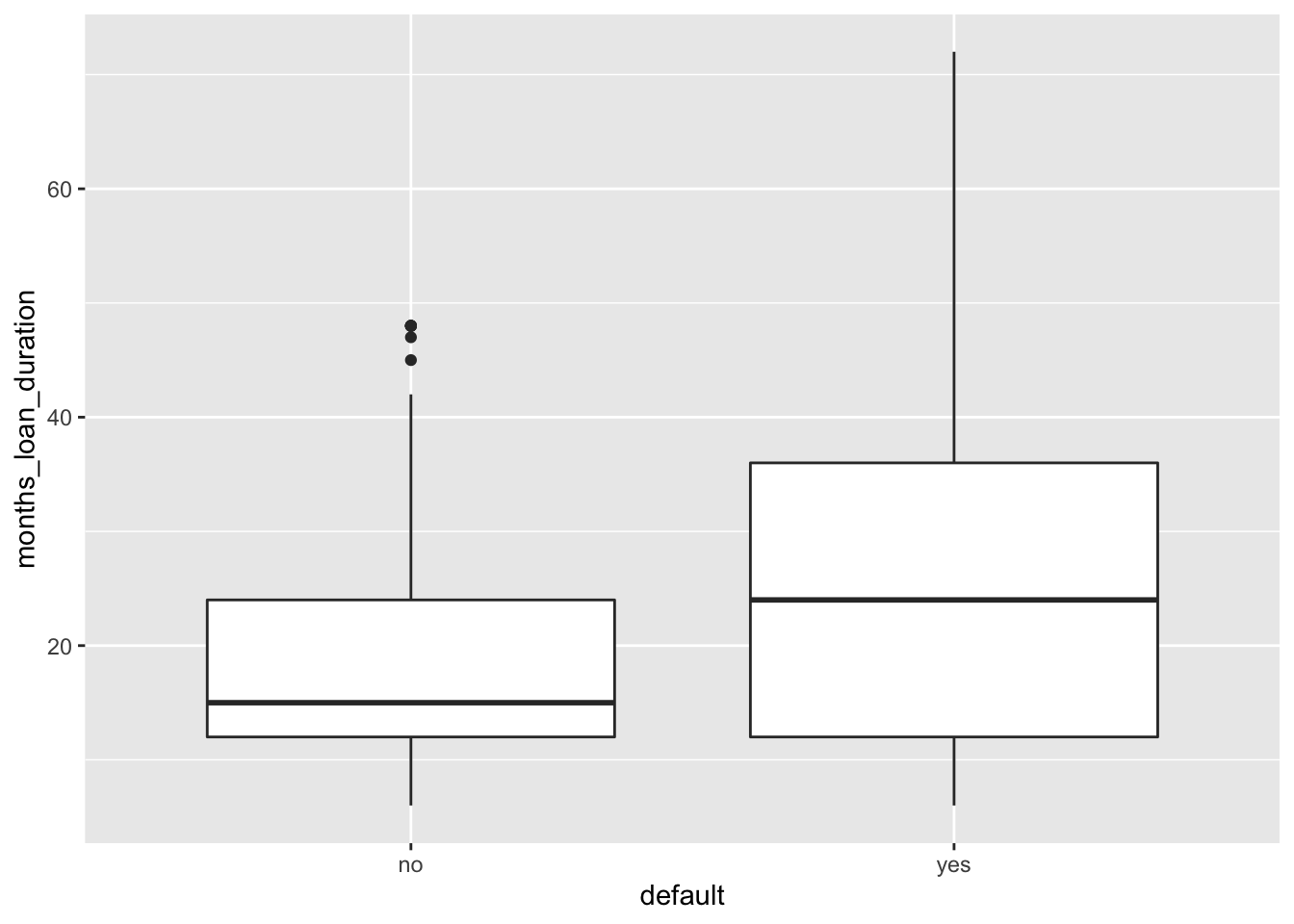
# higher median duration value in case of default

credit %>%
  ggplot()+
  geom_boxplot(aes(x=default, y=age))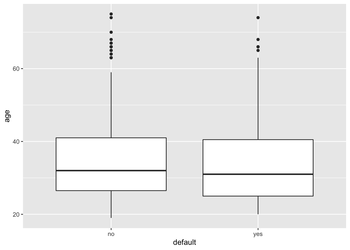
# similar distribution between the two classes for age

credit %>%
  ggplot()+
  geom_bar(aes(x=percent_of_income,fill=default),
                 position="fill") +
  facet_wrap(~years_at_residence)+
  labs(title = "percent_of_income % distribution by default",
       subtitle = "Analysis stratified by years_at_residence ")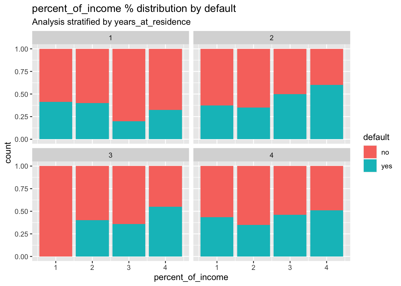
# some small differences in the distribution of the default are visible across the different categories of percent_of_income and years_at_residceWe split the dataset in training (70%) and test set (30%) by using the approach described in Section 2.1.1:
# Create a vector of indexes with an 80% random sample
set.seed(13, sample.kind="Rejection")
train_index = sample(1:nrow(credit), 0.7*nrow(credit))

# Subset the credit data frame to training indexes only
credit_train = credit[train_index, ]
credit_train %>%
  count(default) %>%
  mutate(n/sum(n))
## default n n/sum(n)
## 1 no 204 0.5589041
## 2 yes 161 0.44109595.2 Classification tree
To estimate the classification tree we use the rpart already used before for the grade data. Here the selected method is class as we are dealing with a classification problem. The Gini index will be used for splitting:
## n= 365
##
## node), split, n, loss, yval, (yprob)
##       * denotes terminal node
##
##   1) root 365 161 no (0.5589041 0.4410959)
##     2) months_loan_duration< 47.5 336 137 no (0.5922619 0.4077381)
##       4) months_loan_duration< 17 159  50 no (0.6855346 0.3144654)
##         8) months_loan_duration< 7.5 33   5 no (0.8484848 0.1515152) *
##         9) months_loan_duration>=7.5 126  45 no (0.6428571 0.3571429)
##          18) months_loan_duration>=9.5 106  35 no (0.6698113 0.3301887) *
##          19) months_loan_duration< 9.5 20  10 no (0.5000000 0.5000000)
##            38) age>=32.5 9   2 no (0.7777778 0.2222222) *
##            39) age< 32.5 11   3 yes (0.2727273 0.7272727) *
##       5) months_loan_duration>=17 177  87 no (0.5084746 0.4915254)
##        10) age>=26.5 126  57 no (0.5476190 0.4523810)
##          20) months_loan_duration>=37.5 8   1 no (0.8750000 0.1250000) *
##          21) months_loan_duration< 37.5 118  56 no (0.5254237 0.4745763)
##            42) percent_of_income< 3.5 59  24 no (0.5932203 0.4067797) *
##            43) percent_of_income>=3.5 59  27 yes (0.4576271 0.5423729)
##              86) age< 30.5 21   9 no (0.5714286 0.4285714)
##               172) months_loan_duration< 22.5 7   1 no (0.8571429 0.1428571) *
##               173) months_loan_duration>=22.5 14   6 yes (0.4285714 0.5714286) *
##              87) age>=30.5 38  15 yes (0.3947368 0.6052632)
##               174) months_loan_duration>=25.5 11   4 no (0.6363636 0.3636364) *
##               175) months_loan_duration< 25.5 27   8 yes (0.2962963 0.7037037) *
##        11) age< 26.5 51  21 yes (0.4117647 0.5882353) *
##     3) months_loan_duration>=47.5 29   5 yes (0.1724138 0.8275862) *
It is possible to obtain the size of the tree by counting the number of nodes which are classified as leaf nodes:
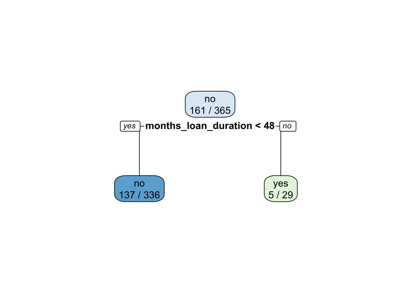
## [1] 12Here below we plot the classification tree by trying also different option of the rpart.plot function (see also http://www.milbo.org/rpart-plot/prp.pdf):
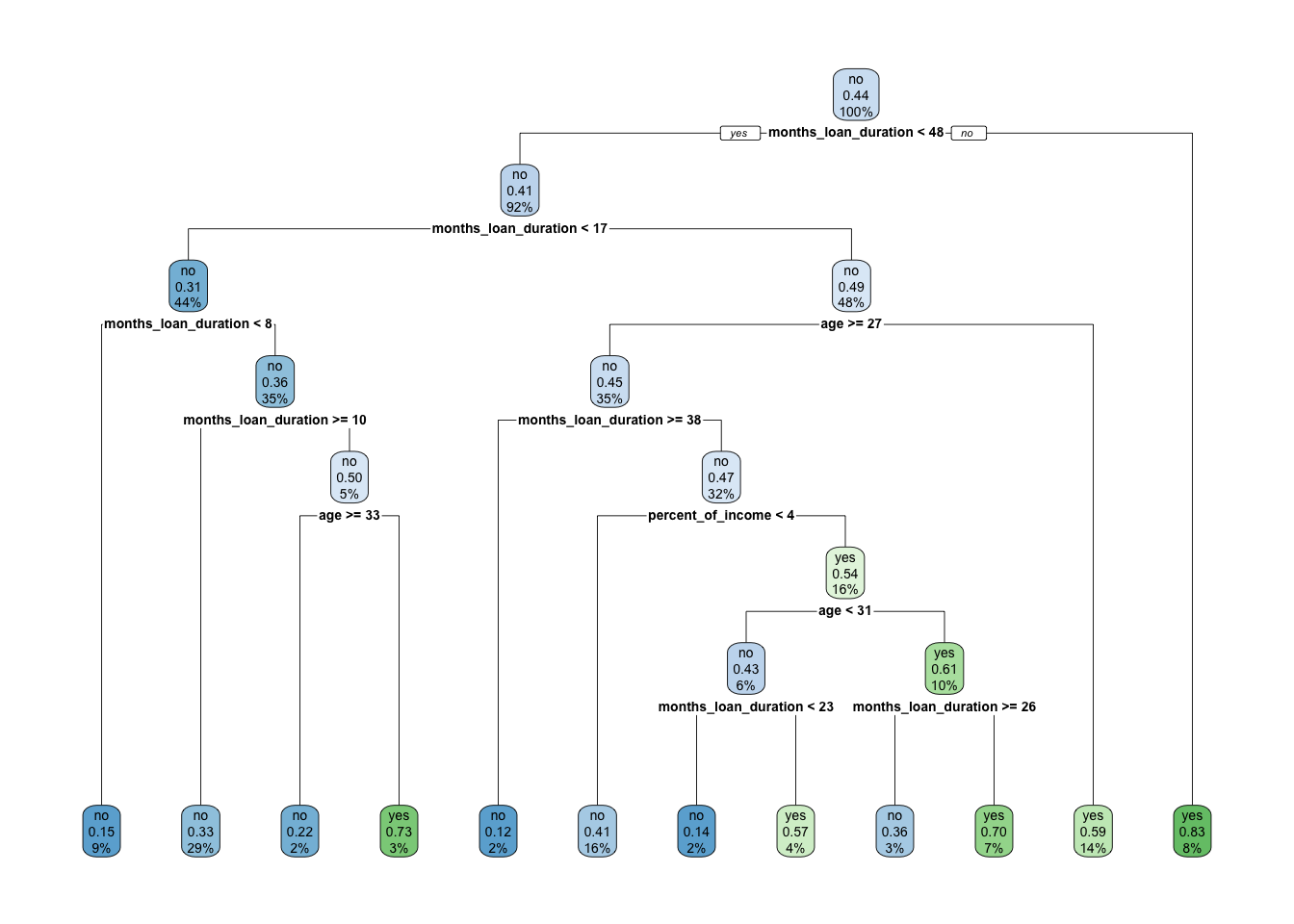
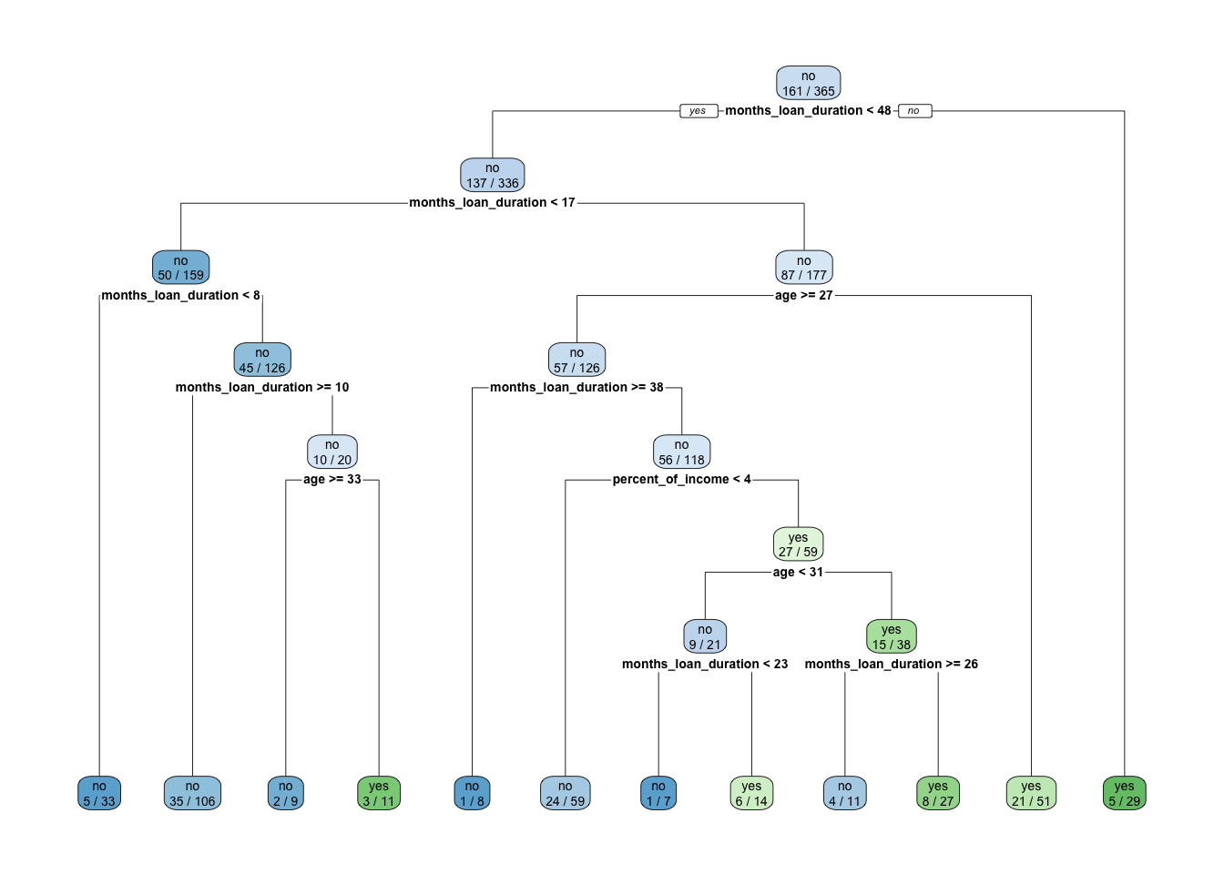
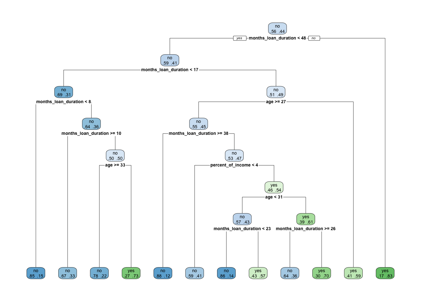
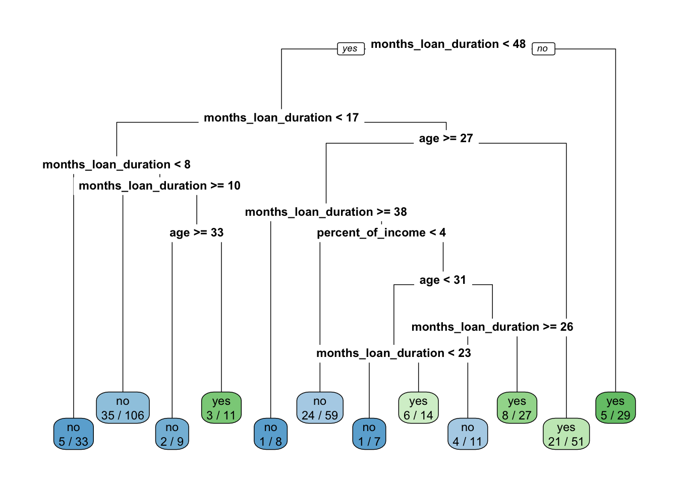
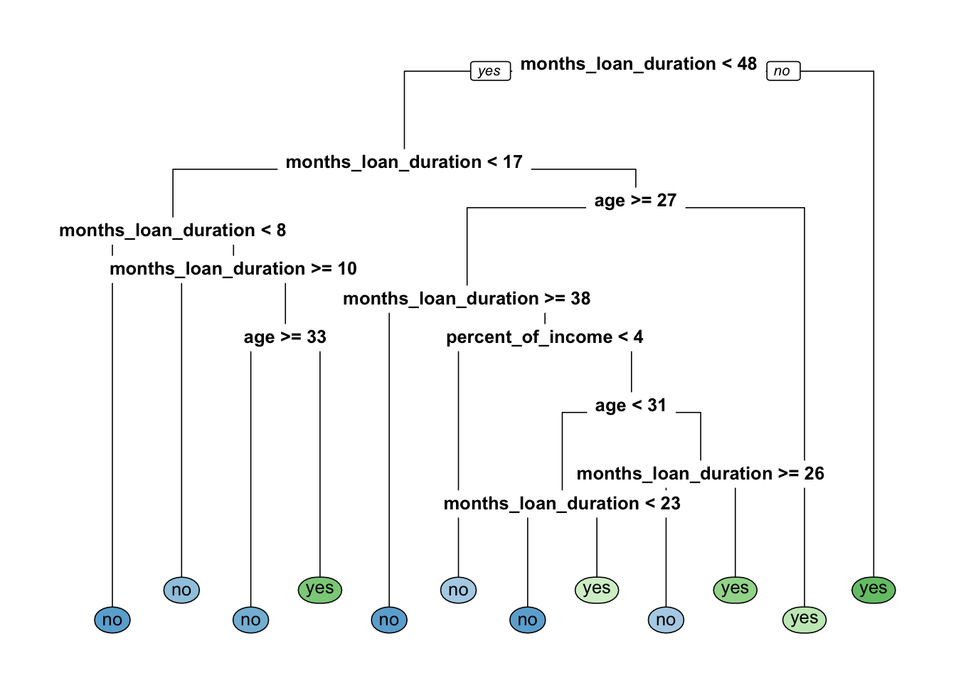
We compute now the predicted category for the observations in the test set:
##   3   6   8  10  11  21
##  no  no  no  no yes  no
## Levels: no yes
Given the predicted category, it is possible to create the confusion matrix and to compute the performance indexes as described in Section 3.2. Here we compute only the accuracy for the sake of simplicity:
##
## credit_treepred no yes
##             no  65  38
## yes 22 32## [1] 0.6178344We see that 61.78% of the test observations are correctly classified. This is quite a poor performance.
As described in Section 4.4, we evaluate the possibility of pruning the tree by using the information contained in the cptable:
##           CP nsplit rel.error    xerror       xstd
## 1 0.11801242      0 1.0000000 1.0000000 0.05891905
## 2 0.02795031      1 0.8819876 0.9316770 0.05838383
## 3 0.01552795      3 0.8260870 1.0496894 0.05916966
## 4 0.01242236      7 0.7577640 1.0186335 0.05902658
## 5 0.01035197      8 0.7453416 0.9875776 0.05883827
## 6 0.01000000 11 0.7142857 1.0124224 0.05899255## [1] 0.02795031In this case the minimum value of the cross-validation error (xerror) corresponds to a very small number of splits (only 1 split). In this case there is no possibility to simplify further the tree, unless we chosse nsplit=0, a choise which is not interesting for us because it means that we are not using any predictor for the credit model. Thus, in this specific case it doesn’t make sense to implement the 1-SE approach described in Section 4.4. We consider directly the value of CP corresponding to the lowest value of xerror and to nsplit=1.
Let’s prune the tree by using the chosen value of CP:
We can now compute the accuracy for the pruned tree:
credit_treepred_prun = predict(credit_tree_prun,
                          newdata = credit_test,
                          type = "class")
table(credit_treepred_prun,
      credit_test$default)
##
## credit_treepred_prun no yes
## no 87 62
## yes 0 8## [1] 0.6050955## [1] 0.6178344The pruned tree is basically a stump and has an accuracy which is basically very similar to the original single tree. Given the similar accuracy, we prefer the pruned tree because it has the advantage of being simpler (or less complex).
We now compute for the selected tree the predicted probabilities that will be required later for the ROC curve:
# Calculate predicted probabilities
credit_treepred_prun_prob = predict(credit_tree_prun,
                               newdata = credit_test,
                               type = "prob")

head(credit_treepred_prun_prob)
## no yes
## 3 0.5922619 0.4077381
## 6 0.5922619 0.4077381
## 8 0.5922619 0.4077381
## 10 0.5922619 0.4077381
## 11 0.5922619 0.4077381
## 21 0.5922619 0.4077381Note that in this case we obtain a matrix with 2 columns (one for each category) and a number of rows given by the number of observations in the test set. For each row the prediction (also reported in the vector credit_treepred_prun) is given by the majority category (i.e. the category with the highest probability).
5.3 Bagging
Bagging has already been described in Section 4.5 for the case of a regression tree. It works similarly for a classification tree:
set.seed(1, sample.kind="Rejection")
credit_bag = randomForest(formula = default ~ .,
                             data = credit_train,
                             mtry = ncol(credit_train)-1, #minus the response
                             importance = T, #to estimate predictors importance
                             ntree = 500) #500 by default
credit_bag
##
## Call:
## randomForest(formula = default ~ ., data = credit_train, mtry = ncol(credit_train) - 1, importance = T, ntree = 500)
## Type of random forest: classification
## Number of trees: 500
## No. of variables tried at each split: 4
##
## OOB estimate of error rate: 46.58%
## Confusion matrix:
## no yes class.error
## no 126 78 0.3823529
## yes 92 69 0.5714286The output provides the out-of-bag (OOB) estimate of the error rate (an unbiased estimate of the test set error) and the corresponding confusion matrix. The former could be used for discriminating between different random forest classifiers (estimated, for example, with different values of ntree).
We analyze now graphically the importance of the regressors (this output is obtained by setting importance = T:
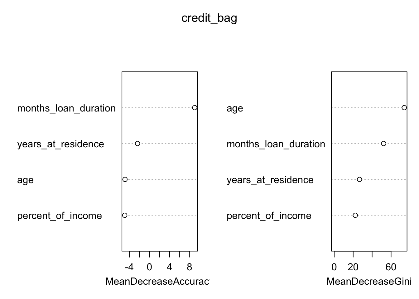
The figure displays:
- in the left plot the mean decrease (across all \(B\) trees) of accuracy in prediction on the OOB samples when a given variable is excluded. This measures how much accuracy the model losses by excluding each variable.
- in the right plot the mean decrease (across all \(B\) trees) in node purity on the OOB samples when a given variable is excluded. For classification, the node impurity is measured by the Gini index. This measures how much each variable contributes to the homogeneity of the nodes in the resulting random forest.
In general the higher the value of the mean decrease accuracy/Gini, the higher the importance of the variable in the model.
For the considered case we see that months_loan_duration and age are the two most important regressors (the former was used also in the single pruned tree).
We compute now the predictions and the test confusion matrix and accuracy given by bagging:
##   3   6   8  10  11  21
##  no  no  no  no yes  no
## Levels: no yes## [1] 0.6050955## [1] 0.5605096By comparing accuracy, bagging performs slightly worse with respect to the single prune tree.
We also compute the predicted probabilities that will be needed later:
5.4 Random forest
Random forest is very similar to bagging. The only difference is in the specification of the mtry argument. For a classification problem we consider a number of regressors to be selected randomly to be equal to \(\sqrt{p}\):
set.seed(1, sample.kind="Rejection")
credit_rf = randomForest(formula = default ~ .,
                             data = credit_train,
                             mtry = sqrt(ncol(credit_train)-1),
                             importance = T,
                             ntree = 500)
print(credit_rf)
##
## Call:
## randomForest(formula = default ~ ., data = credit_train, mtry = sqrt(ncol(credit_train) - 1), importance = T, ntree = 500)
## Type of random forest: classification
## Number of trees: 500
## No. of variables tried at each split: 2
##
## OOB estimate of error rate: 46.03%
## Confusion matrix:
## no yes class.error
## no 131 73 0.3578431
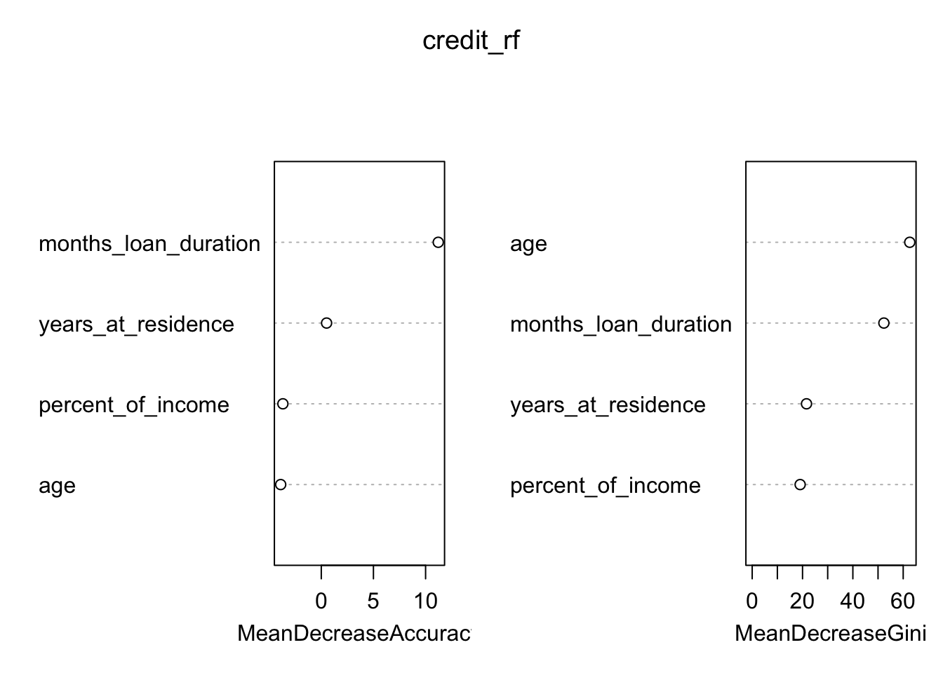
## yes 95 66 0.5900621As before we plot the measure for the importance of the regressors:
Finally, we compute the predictions of default by using the random forest model:
credit_rfpred = predict(object = credit_rf,
                            newdata = credit_test,
                            type = "class")

# Calculate the confusion matrix for the test set
table(credit_test$default, credit_rfpred)
## credit_rfpred
## no yes
## no 65 22
## yes 42 28## [1] 0.6050955## [1] 0.5605096## [1] 0.5923567# Compute predicted probabilities
credit_rf_pred_prob = predict(object = credit_rf,
newdata = credit_test,
type = "prob")By comparing accuracy, we conclude the random forest performs better than bagging and similarly to the single pruned tree. However, all the accuracies are very low.
5.5 Model comparison by using the ROC curves
By using the ROC curve introduced in Section 3.7, we compute the implemented models for the credit problem:
## Setting levels: control = no, case = yes## Setting direction: controls < cases## Setting levels: control = no, case = yes
## Setting direction: controls < cases## Setting levels: control = no, case = yes
## Setting direction: controls < casesThen we plot them all in the same plot:
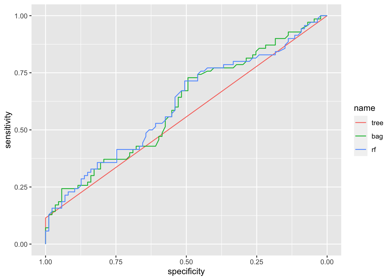
Note that the roc curve for the single tree is practically a straight line. This is basically due to the fact that the single tree is a stump and specificity/sensitivity (computed using predictions) don’t change that much by modification of the probability threshold. The bagging and random forest roc curves are very similar.
Finally we compute the area under the curve (AUC) for the three methods:
## Area under the curve: 0.5571## Area under the curve: 0.6071## Area under the curve: 0.6099All the AUC values are very similar and all very low. They denote a poor performance of all the classifiers. I think this is a problem mainly related to the regressors that are used in the analysis which are not informative enough for describing the pattern of the default variable.
5.6 Exercises Lab 4
5.6.1 Exercise 1
We use the OJ dataset which is part of the ISLR library. The data refers to 1070 purchases where the customer either purchased Citrus Hill (CH) or Minute Maid Orange Juice (MM). The response variable is Purchase. A number of characteristics of the customers are recorded (see ?OJ).
## [1] 1070 18## Rows: 1,070
## Columns: 18
## $ Purchase <fct> CH, CH, CH, MM, CH, CH, CH, CH, CH, CH, CH, CH, CH, CH,…
## $ WeekofPurchase <dbl> 237, 239, 245, 227, 228, 230, 232, 234, 235, 238, 240, …
## $ StoreID <dbl> 1, 1, 1, 1, 7, 7, 7, 7, 7, 7, 7, 7, 7, 7, 7, 7, 1, 2, 2…
## $ PriceCH <dbl> 1.75, 1.75, 1.86, 1.69, 1.69, 1.69, 1.69, 1.75, 1.75, 1…
## $ PriceMM <dbl> 1.99, 1.99, 2.09, 1.69, 1.69, 1.99, 1.99, 1.99, 1.99, 1…
## $ DiscCH <dbl> 0.00, 0.00, 0.17, 0.00, 0.00, 0.00, 0.00, 0.00, 0.00, 0…
## $ DiscMM <dbl> 0.00, 0.30, 0.00, 0.00, 0.00, 0.00, 0.40, 0.40, 0.40, 0…
## $ SpecialCH <dbl> 0, 0, 0, 0, 0, 0, 1, 1, 0, 0, 0, 0, 0, 0, 0, 0, 0, 0, 0…
## $ SpecialMM <dbl> 0, 1, 0, 0, 0, 1, 1, 0, 0, 0, 0, 0, 1, 0, 0, 0, 1, 1, 0…
## $ LoyalCH <dbl> 0.500000, 0.600000, 0.680000, 0.400000, 0.956535, 0.965…
## $ SalePriceMM <dbl> 1.99, 1.69, 2.09, 1.69, 1.69, 1.99, 1.59, 1.59, 1.59, 1…
## $ SalePriceCH <dbl> 1.75, 1.75, 1.69, 1.69, 1.69, 1.69, 1.69, 1.75, 1.75, 1…
## $ PriceDiff <dbl> 0.24, -0.06, 0.40, 0.00, 0.00, 0.30, -0.10, -0.16, -0.1…
## $ Store7 <fct> No, No, No, No, Yes, Yes, Yes, Yes, Yes, Yes, Yes, Yes,…
## $ PctDiscMM <dbl> 0.000000, 0.150754, 0.000000, 0.000000, 0.000000, 0.000…
## $ PctDiscCH <dbl> 0.000000, 0.000000, 0.091398, 0.000000, 0.000000, 0.000…
## $ ListPriceDiff <dbl> 0.24, 0.24, 0.23, 0.00, 0.00, 0.30, 0.30, 0.24, 0.24, 0…
## $ STORE <dbl> 1, 1, 1, 1, 0, 0, 0, 0, 0, 0, 0, 0, 0, 0, 0, 0, 1, 2, 2…- Create a training set containing a random sample of 800 observations (use as seed the value 4455) and a test set containing the remaining observations.
- Consider
Purchaseas response variable. Provide and plot its frequency distribution for the training observations. - Fit a tree to the training data for
Purchase. Use all the other variables as predictors.Plot the tree. Which is the most important variable? Try different specifications of the
extraandtypeargument of therpart.plotfunction (see?rpart.plot)Extract all the information available for observation n. 146 in the training data set. Which is the
Purchaseprediction for this observation using the estimated tree?Predict the response for the test data and produce a confusion matrix. What is the test errorr rate?
- Do you think is it convenient to prune the tree? If yes, estimate the pruned tree and plot it.
- If you decided to prune the tree, compute the test error rate for the pruned tree. Compare the test error rate of the pruned and unpruned tree. Which is better?
5.6.2 Exercise 2
Consider the BreastCancer dataset included in the mlbench library.
## Rows: 699
## Columns: 11
## $ Id              <chr> "1000025", "1002945", "1015425", "1016277", "1017023",…
## $ Cl.thickness    <ord> 5, 5, 3, 6, 4, 8, 1, 2, 2, 4, 1, 2, 5, 1, 8, 7, 4, 4, …
## $ Cell.size       <ord> 1, 4, 1, 8, 1, 10, 1, 1, 1, 2, 1, 1, 3, 1, 7, 4, 1, 1,…
## $ Cell.shape      <ord> 1, 4, 1, 8, 1, 10, 1, 2, 1, 1, 1, 1, 3, 1, 5, 6, 1, 1,…
## $ Marg.adhesion   <ord> 1, 5, 1, 1, 3, 8, 1, 1, 1, 1, 1, 1, 3, 1, 10, 4, 1, 1,…
## $ Epith.c.size    <ord> 2, 7, 2, 3, 2, 7, 2, 2, 2, 2, 1, 2, 2, 2, 7, 6, 2, 2, …
## $ Bare.nuclei     <fct> 1, 10, 2, 4, 1, 10, 10, 1, 1, 1, 1, 1, 3, 3, 9, 1, 1, …
## $ Bl.cromatin     <fct> 3, 3, 3, 3, 3, 9, 3, 3, 1, 2, 3, 2, 4, 3, 5, 4, 2, 3, …
## $ Normal.nucleoli <fct> 1, 2, 1, 7, 1, 7, 1, 1, 1, 1, 1, 1, 4, 1, 5, 3, 1, 1, …
## $ Mitoses         <fct> 1, 1, 1, 1, 1, 1, 1, 1, 5, 1, 1, 1, 1, 1, 4, 1, 1, 1, …
## $ Class           <fct> benign, benign, benign, benign, benign, malignant, ben…
Remove missing values and the variable named
Id(identifier), which is useless and would confuse the machine learning algorithms.Partition the data set for 80% training and 20% evaluation (seed=2).
Use the training data for growing a tree for predicting
Classas a function of all the other variables. Plot the tree.Compute the predictions (classes and probabilities, separately) for the test observations. Compute the accuracy.
Implement bagging and compare its performance (in terms of accuracy) with the full classification tree implemented before. Compute also probabilities that will be used at the end for the AUC.
Implement random forest and compare its performance (in terms of accuracy) with the methods implemented before. Compute also probabilities that will be used at the end for the AUC.
For all the considered models compute the AUC and plot the ROCs.