1 Introduction to Forecasting
A forecast us a prediction of some future event or events. As suggested by Neils Bohr, making good predictions is not always easy. Famously “bad” forecasts include the following from the book Bad Predictions:
- “The population is constant in size and will remain so right up to the end of mankind” L’Encyclopedie, 1756.
- “1930 will be a splendid employment year.” U.S. Department of Labor, New Year’s Forecast in 1929, just before the market crash on October 29.
- “Computers are multiplying at a rapid rate. By the turn of the century there will be 220,000 in the U.S.” Wall Street Journal, 1966.
Forecasting problems occur in many fields:
- business
- economics
- finance
- environmental science
- social sciences
- political sciences
Forecasting Problems:
- Short-term
- Predicting only a few periods ahead (hours, days, weeks)
- Typically based on modeling and extrapolating patterns in the data
- Medium-Term
- One to two years into the future, typically
- Long-Term
- several years into the future
Many business applications of forecasting utilize daily, weekly, monthly, quarterly, or annual data, but any reporting interval may be used.
The data may be instantaneous, such as the viscosity of a chemical product at the point in time where it is measured; it may be cumulative, such as the total sales of a product during the month; or it may be a statistic that in some way reflects the activity of the variable during the time period, such as the daily closing price of a specific stock on the New York Stock Exchange.
The reason that forecasting is so important is that prediction of future events is a critical input into many types of planning and decision making processes, with application to areas such as the following:
- Operations Management. Business organizations routinely use forecasts of product sales or demand for services in order to schedule production, control inventories, manage the supply chain, determine staffing requirements, and plan capacity. Forecasts may also be used to determine the mix of products or services to be offered and the locations at which products are to be produced.
- Marketing. Forecasting is important in many marketing decisions. Forecasts of sales response to advertising expenditures, new promotions, or changes in pricing policies enable businesses to evaluate their effectiveness, determine whether goals are being met, and make adjustments.
- Finance and Risk Management. Investors in financial assets are interested in forecasting the returns from their investments. These assets include but are not limited to stocks, bonds, and commodities; other investment decisions can be made relative to forecasts of internal rates, options, and currency exchange rates. Financial risk management requires forecast of the volatility of asset returns so that the risks associated with investment portfolios can be evaluated and insured, and so that financial derivatives can be properly priced.
- Economics. Governments, financial institutions, and policy organizations require forecasts of major economic variables, such as gross domestic product, population growth, unemployment, interest rates, inflation, job growth, production, and consumption. These forecasts are an integral part of the guidance behind monetary and fiscal policy and budgeting plans and decisions made by governments. They are also instrumental in the strategic planning decisions made by business organizations and financial institutions.
- Industrial Process Control. Forecasts of future values of critical quality characteristics of a production process can help determine when important controllable variables in the process should be changed, or if the process should be shut down and overhauled. Feedback and feedforward control schemes are widely used in monitoring and adjustment of industrial processes, and predictions of the process output are an integral part of these schemes.
- Demography. Forecasts of population by country and regions are med routinely, often stratified by variables such as gender, age, and race. Demographers also forecast births, deaths, and migration patterns of populations. Governments use these forecasts for planning policy and social service actions, such as spending on health care, retirement programs, and antipoverty programs. Many businesses use forecasts of populations by age groups to make strategic plans regarding developing new product lines or the types of services that will be offered.
Two types of methods:
- Quantitative forecasting methods
- Makes formal use of historical data
- A mathematical/statistical model
- Past patterns are modeled and projected into the future
- Qualitative forecasting methods
- Subjective
- Little available data (new product introduction)
- Expert opinion often used
- The Delphi method
Quantitative forecasting methods:
- Regression methods
- Sometimes called causal methods
- Chapter 3
- Smoothing methods
- Often justified empirically
- Chapter 4
- Formal time series analysis methods
- Chapters 5 and 6
- Some other related methods are discussed in Chapter 7
Terminology:
- Point forecast or point estimate
- Prediction interval
- Forecast horizon or lead time
- Forecasting interval
- Moving horizon forecasts
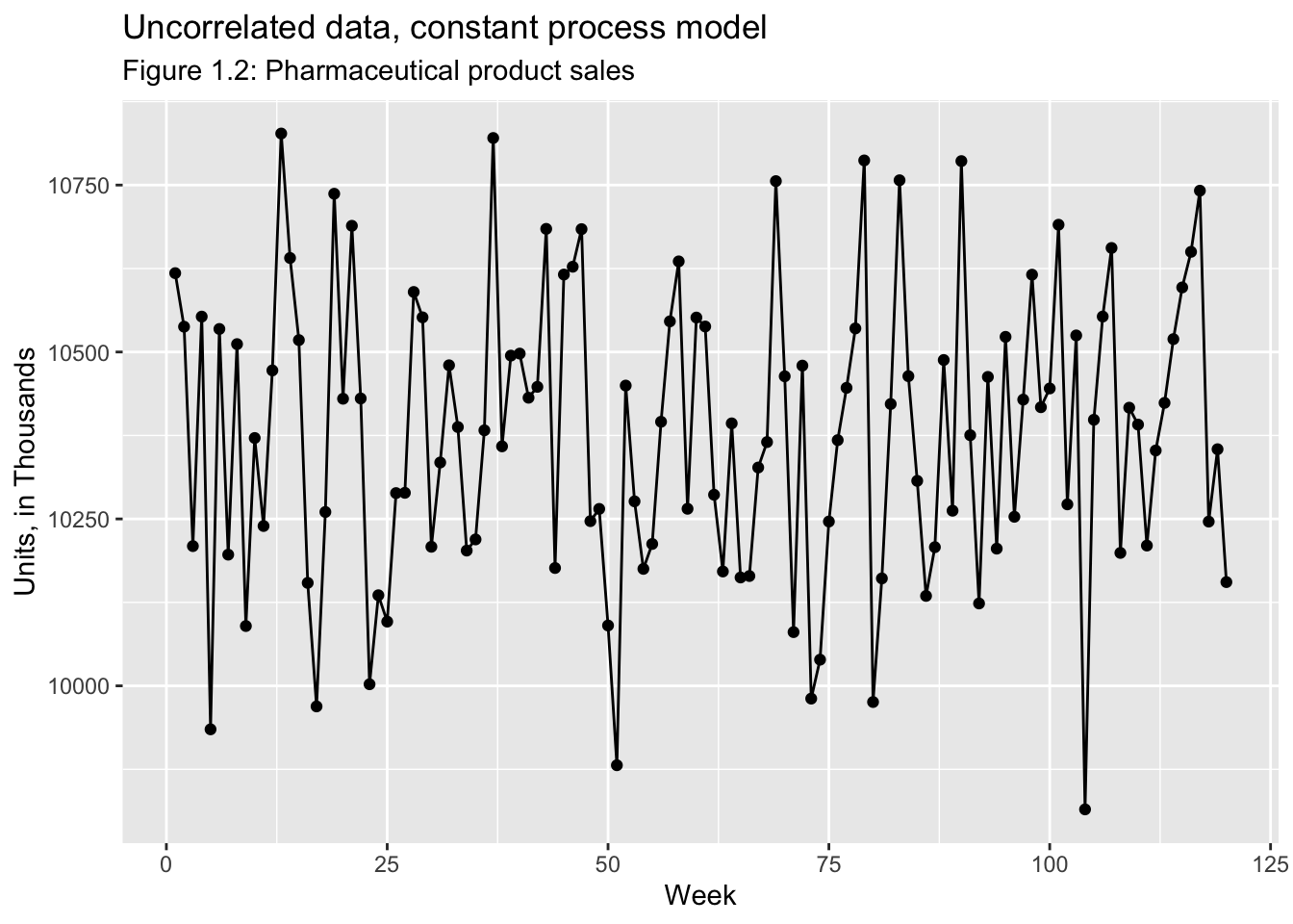
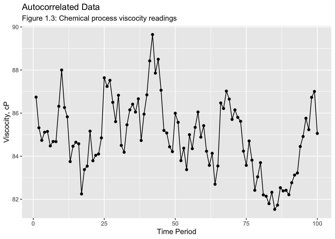
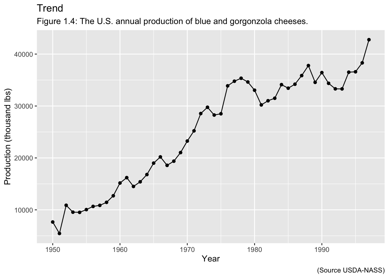
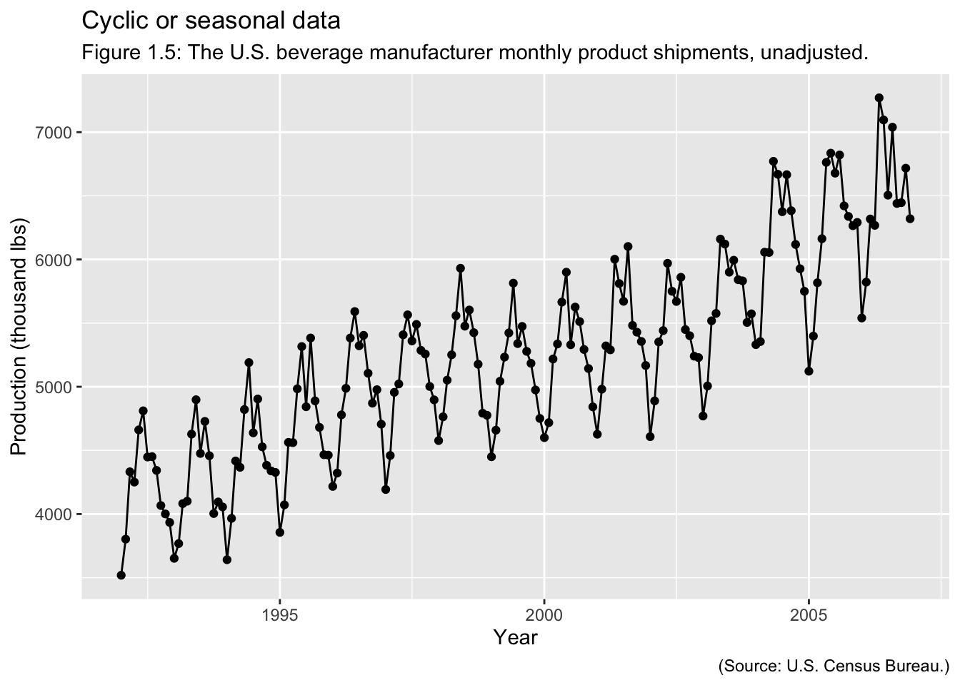
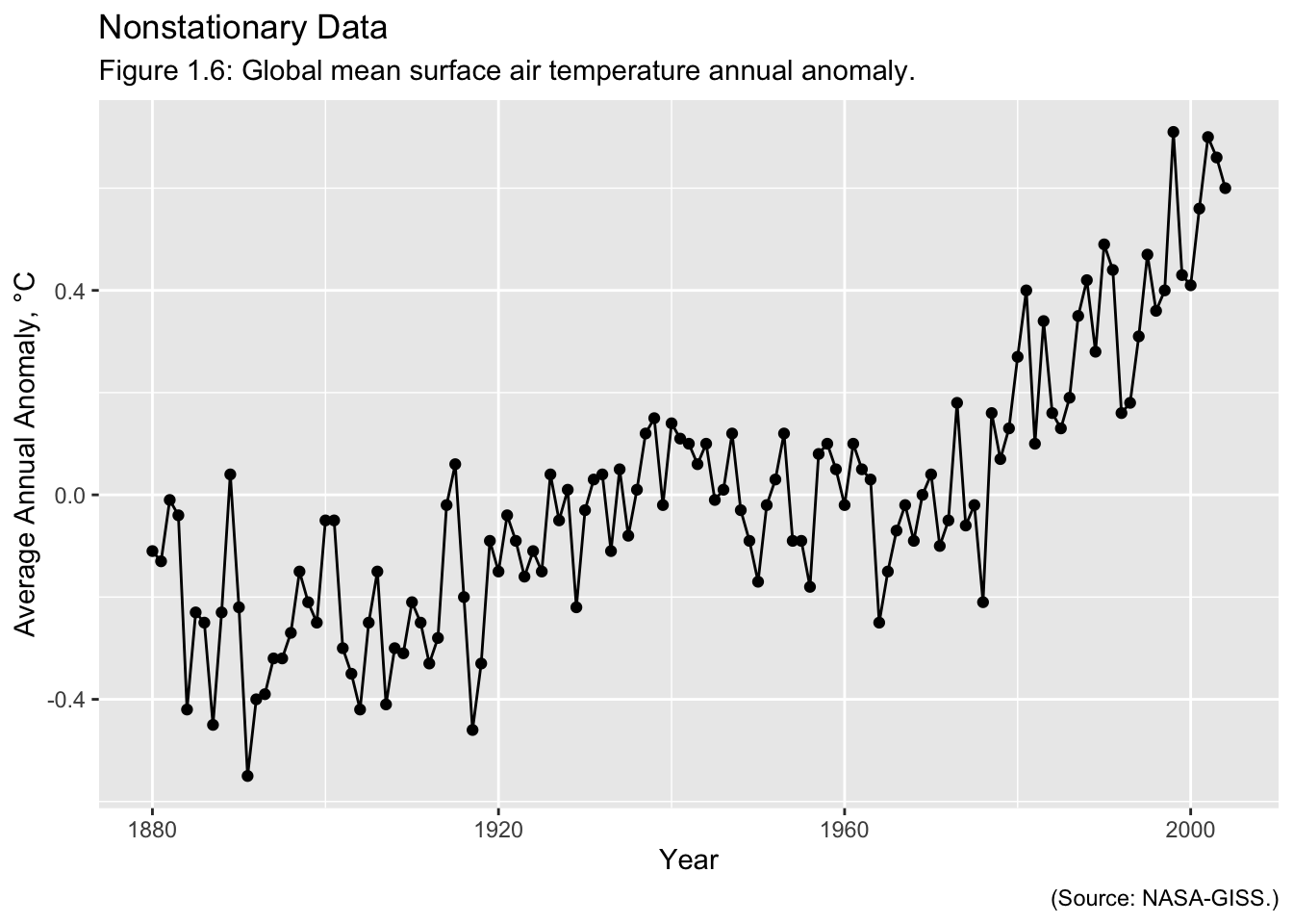
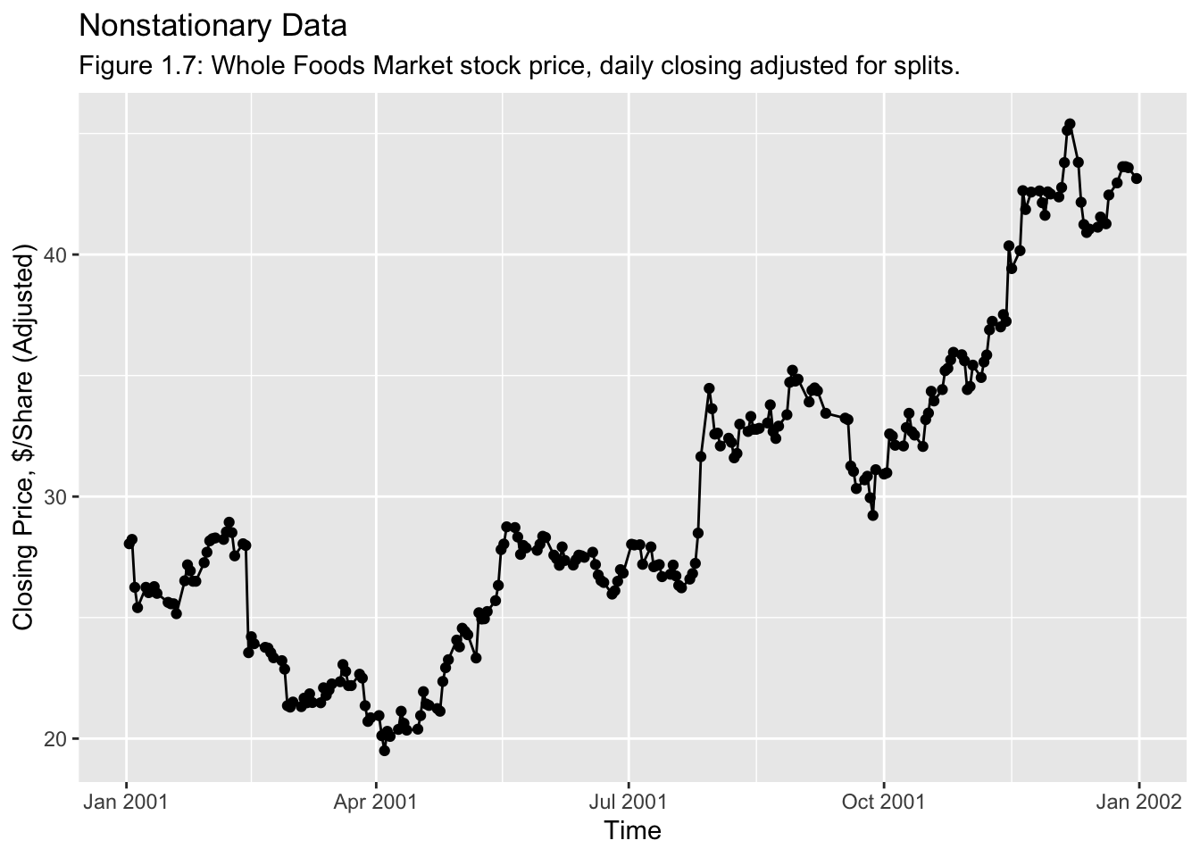
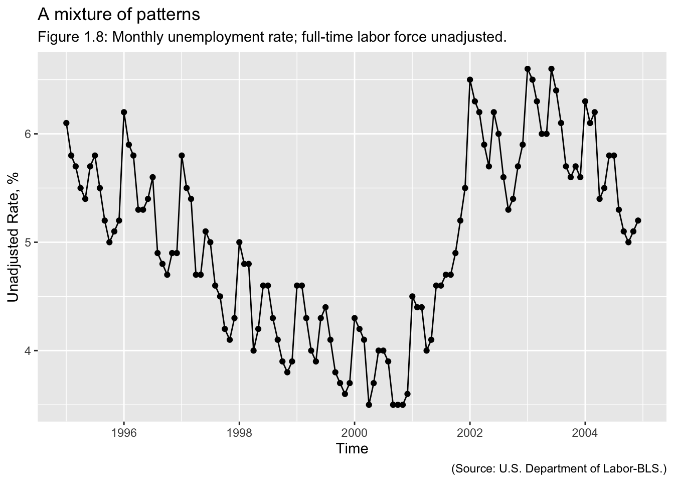
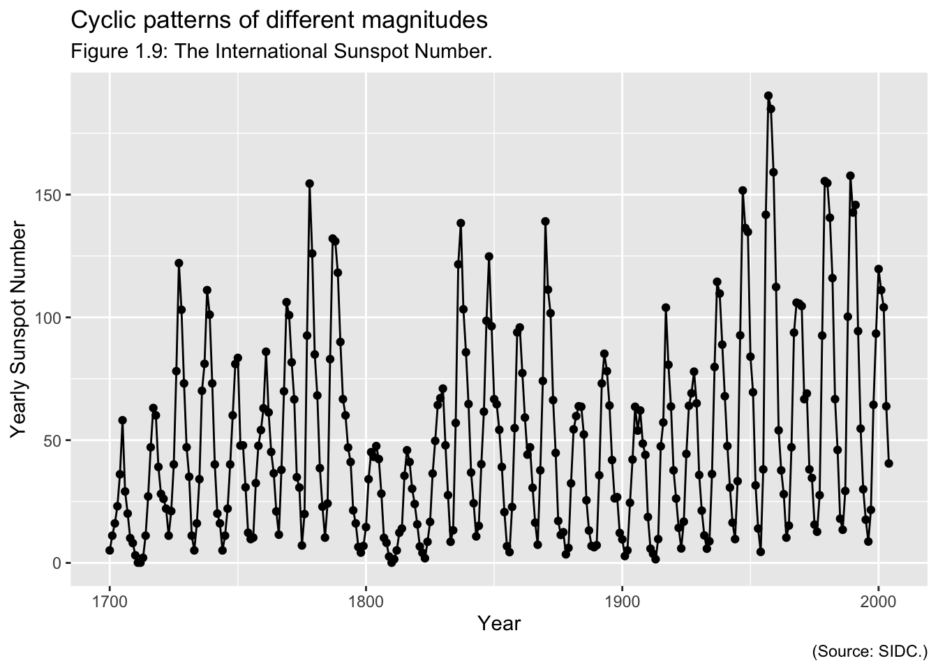
Examples of Time Series:
The Forecasting Process: A process is a series of connected activities that transform one or more inputs into one or more outputs. All work activities are performed in processes, and forecasting is no exception. The activities in the forecasting process are:
- Problem definition
- Data collection
- Data analysis
- Model selection and fitting
- Model validation
- Forecasting model development
- Monitoring forecasting model performance
Data for Forecasting
- The Data Warehouse
- Data versus information
- In most modern organizations, data regarding sales, transactions, company financial and business performance, supplier performance, and customer activity and relations are stored in a repository known as a data warehouse. Sometimes this is a single data storage system; but as the volume of data handled by modern organizations grows rapidly, the data warehouse had become an integrated system comprised of components that are physically and often geographically distributed, such a cloud data storage. The data warehouse must be able to organize, manipulate, and integrate data from multiple sources and different organizational information systems.
Required Functionality
- data extraction
- data transformation
- duplication of records
- missing data
- other problems
- sometimes called data cleaning
- data loading
Data Quality
- accuracy
- timeliness
- completeness
- representativeness
- consistency
- Jones-Farmer et al. (2014) describe how statistical quality control methods (specifically control charts) can be used to enhance data quality in the data production process.
Data Cleaning
- Looking for and fixing potential errors, missing data, outliers, inconsistencies
- Some common “automatic” checks include:
- Is data missing?
- Does the data fall within expected ranges?
- Are there outliers or unusual values?
- Graphical as well as analytical methods can be useful.
Data Imputation
- Correcting missing values
- Mean value imputation
- Stochastic mean value imputation
- Mean value imputation using a subset of the data
- Regression imputation
- The imputed value is computed from a model
- “Hot deck” imputation
- uses the data currently available
- “Cold deck” imputation
- uses other data not currently in use
1.1 Time Series Objects
For this class, we will be using the fpp3 set of packages that accompany Rob Hyndman’s Forecasting: Principles and Practice.12 In the code chunk below, I load fpp3 as well as the tidyverse and read_xl. These packages provide any functions I might need in the data importing, wrangling, and cleaning process.
## ── Attaching packages ───────────────────────────── fpp3 0.5 ──## ✔ tsibble 1.1.3 ✔ fable 0.3.3
## ✔ tsibbledata 0.4.1 ✔ fabletools 0.3.3
## ✔ feasts 0.3.1## ── Conflicts ──────────────────────────────── fpp3_conflicts ──
## ✖ lubridate::date() masks base::date()
## ✖ dplyr::filter() masks stats::filter()
## ✖ tsibble::intersect() masks base::intersect()
## ✖ tsibble::interval() masks lubridate::interval()
## ✖ dplyr::lag() masks stats::lag()
## ✖ tsibble::setdiff() masks base::setdiff()
## ✖ tsibble::union() masks base::union()Hyndman uses tsibble() objects to create time series objects within R.13 These objects are like tibbles, in that they are able to be manipulated by dplyr functions and can store multiple variables. The additional index = parameter allows you to set the index equal to the time variable.14 In the code chunk below, I import Appendix B.5 Table of U.S. beverage manufacturer product shipments, unadjusted.15. This will be made into a tsibble as an example. I use read_excel() to import the data, rename() to appropriately name the variables for coding, and mutate() to correctly specify the time variable with the function yearmonth().
bev <- read_excel("data/bev.xlsx", skip = 3) |>
  rename(time = Month, dollars = `Dollars, in Millions`) |>
  mutate(time = yearmonth(time))
bev
## # A tibble: 180 × 2
## time dollars
## <mth> <dbl>
## 1 1992 Jan 3519
## 2 1992 Feb 3803
## 3 1992 Mar 4332
## 4 1992 Apr 4251
## 5 1992 May 4661
## 6 1992 Jun 4811
## 7 1992 Jul 4448
## 8 1992 Aug 4451
## 9 1992 Sep 4343
## 10 1992 Oct 4067
## # ℹ 170 more rowsThere are two main ways to create a tsibble: tsibble() or as_tsibble(). as_tsibble() converts an existing data frame, such as the bev data frame saved in the code chunk above, into a tsibble. The index = argument must be used to denote which variable represents time. This is demonstrated in the code chunk below.
## # A tsibble: 180 x 2 [1M]
##        time dollars
##       <mth>   <dbl>
##  1 1992 Jan    3519
##  2 1992 Feb    3803
##  3 1992 Mar    4332
##  4 1992 Apr    4251
##  5 1992 May    4661
##  6 1992 Jun    4811
##  7 1992 Jul    4448
##  8 1992 Aug    4451
##  9 1992 Sep    4343
## 10 1992 Oct    4067
## # ℹ 170 more rows
The tsibble() function operates similarly to the tibble() function. Each variable name is set equal to the corresponding vector of values and the index is specified. The code chunk below demonstrates how to use tsibble().
## # A tsibble: 180 x 2 [1M]
##        time dollars
##       <mth>   <dbl>
##  1 1992 Jan    3519
##  2 1992 Feb    3803
##  3 1992 Mar    4332
##  4 1992 Apr    4251
##  5 1992 May    4661
##  6 1992 Jun    4811
##  7 1992 Jul    4448
##  8 1992 Aug    4451
##  9 1992 Sep    4343
## 10 1992 Oct    4067
## # ℹ 170 more rows
The top line of the output, after A tsibble:, contains the important information about the time series. In the example above, 180 refers to the number of observations, 2 refers to the number of rows, and [1M] refers to the frequency of observations (every month). Making all the data you import into tsibble objects allows you to fully take advantage of the fable packages as well as the functions available through the tidyverse. Always check to make sure the tsibble is correctly specified so that it accurately represents your data. For further reference, refer to this Forecasting: Principles and Practice chapter on tsibble objects and the accompanying video.16
1.1.1 Data Importing Examples
This section will provide further examples of how to import data using data files from Introduction to Time Series Analysis and Forecasting.
1.1.1.1 UKmiles.csv
The first example uses the UKmiles.csv file. The first step whenever importing data is to identify the frequency of the data, the index variable, and if anything needs to be changed so the data can be made into a tsibble object using as_tsibble(). The best way to do this is to look at the data immediately after it is imported.
## Rows: 84 Columns: 2
## ── Column specification ───────────────────────────────────────
## Delimiter: ","
## chr (1): month
## dbl (1): miles
##
## ℹ Use `spec()` to retrieve the full column specification for this data.
## ℹ Specify the column types or set `show_col_types = FALSE` to quiet this message.
## # A tibble: 84 × 2
## month miles
## <chr> <dbl>
## 1 Jan-64 7.27
## 2 Feb-64 6.78
## 3 Mar-64 7.82
## 4 Apr-64 8.37
## 5 May-64 9.07
## 6 Jun-64 10.2
## 7 Jul-64 11.0
## 8 Aug-64 10.9
## 9 Sep-64 10.3
## 10 Oct-64 9.11
## # ℹ 74 more rowsLooking at the data imported above, the frequency of observations is monthly and the index variable, month, is stored as a chr type. The month variable must be formatted so it can be set as the index. The tsibble package has a set of functions to create time variables compatible with tsibbles for different frequencies:
yearmonth()- used with monthly data
yearweek()- used with weekly data
yearquarter()- used with quarterly data
Each of these functions has a version with make_ in front (e.g. make_yearmonth(year = , month = )) which can accept different variables as the month and year components of the time object. If the data is more frequent than weekly, either date or datetime objects can be used.
If you were to run the commented code below and try to use yearmonth() to make the month variable into an acceptable type, you would get an error message saying it cannot be expressed as a date type. This is because the year is expressed as only the last 2 digits and yearmonth() requires all four digits. This is a common issue with data in this class.
To correct the month variable, I need to add 19 between the dash and the two digits indicating the year. To do this, I will use two functions from the stringr package:
str_c()- This function concatenates the string elements into a single string in the order listed
str_sub(string, start = , end = )- This function selects a subset of a string by index, specified through
start =andend = - recall indexing starts at 1 in R
- This function selects a subset of a string by index, specified through
The stringr package is included in the tidyverse, so these functions can be used within mutate() to modify all the observations of a variable. In the code chunk below, I demonstrate these function on their own.
## [1] "Hello"## [1] "He"Using the function discussed above, I then modify the month variable by placing "19" between the 4th and 5th index of the month string. Even though the month is in front of the year in this format yearmonth() is still able to parse the variable. yearmonth() must be used after the changes in the first mutate() so I pipe the results into a second mutate where I create a time variable that can be used as the index. As a convention, I almost always name the index variable time.
read_csv("data/UKmiles.csv") |>
  mutate(month = str_c(str_sub(month, start = 1, end = 4),
                       "19",
                       str_sub(month, start = 5, end = 6))) |>
  mutate(time = yearmonth(month))
## Rows: 84 Columns: 2
## ── Column specification ───────────────────────────────────────
## Delimiter: ","
## chr (1): month
## dbl (1): miles
##
## ℹ Use `spec()` to retrieve the full column specification for this data.
## ℹ Specify the column types or set `show_col_types = FALSE` to quiet this message.## # A tibble: 84 × 3
## month miles time
## <chr> <dbl> <mth>
## 1 Jan-1964 7.27 1964 Jan
## 2 Feb-1964 6.78 1964 Feb
## 3 Mar-1964 7.82 1964 Mar
## 4 Apr-1964 8.37 1964 Apr
## 5 May-1964 9.07 1964 May
## 6 Jun-1964 10.2 1964 Jun
## 7 Jul-1964 11.0 1964 Jul
## 8 Aug-1964 10.9 1964 Aug
## 9 Sep-1964 10.3 1964 Sep
## 10 Oct-1964 9.11 1964 Oct
## # ℹ 74 more rowsNow, that I have created a series of functions which imports the data, cleans the data and then stores it as a tibble with the proper index, I can save the result. In the code chunk below, I use the exact same procedure to clean the data as the code chunk above, select only the time variable and the variable of interest, and then save the results as a tsibble.
(UK_miles <- read_csv("data/UKmiles.csv") |>
  mutate(month = str_c(str_sub(month, start = 1, end = 4),
                       "19",
                       str_sub(month, start = 5, end = 6))) |>
  mutate(time = yearmonth(month)) |>
  select(time, miles) |>
  as_tsibble(index = time))
## Rows: 84 Columns: 2
## ── Column specification ───────────────────────────────────────
## Delimiter: ","
## chr (1): month
## dbl (1): miles
##
## ℹ Use `spec()` to retrieve the full column specification for this data.
## ℹ Specify the column types or set `show_col_types = FALSE` to quiet this message.## # A tsibble: 84 x 2 [1M]
## time miles
## <mth> <dbl>
## 1 1964 Jan 7.27
## 2 1964 Feb 6.78
## 3 1964 Mar 7.82
## 4 1964 Apr 8.37
## 5 1964 May 9.07
## 6 1964 Jun 10.2
## 7 1964 Jul 11.0
## 8 1964 Aug 10.9
## 9 1964 Sep 10.3
## 10 1964 Oct 9.11
## # ℹ 74 more rows1.1.1.2 Viscocity
The next example uses data from the Viscosity.csv file. While the file has more than two columns, there are only two variables in the data set, time and reading. This manifests as additional columns containing NA to time and reading. These data do not have an identified frequency. Instead of each observation of time containing a time or date, the first observation has a value of 1 and continues upward. This is called a periodic time variable.
## New names:
## Rows: 100 Columns: 8
## ── Column specification
## ─────────────────────────────────────── Delimiter: "," dbl
## (2): time, reading lgl (6): ...3, ...4, ...5, ...6, ...7, ...8
## ℹ Use `spec()` to retrieve the full column specification for
## this data. ℹ Specify the column types or set `show_col_types =
## FALSE` to quiet this message.
## • `` -> `...3`
## • `` -> `...4`
## • `` -> `...5`
## • `` -> `...6`
## • `` -> `...7`
## • `` -> `...8`
## # A tibble: 100 × 8
## time reading ...3 ...4 ...5 ...6 ...7 ...8
## <dbl> <dbl> <lgl> <lgl> <lgl> <lgl> <lgl> <lgl>
## 1 1 86.7 NA NA NA NA NA NA
## 2 2 85.3 NA NA NA NA NA NA
## 3 3 84.7 NA NA NA NA NA NA
## 4 4 85.1 NA NA NA NA NA NA
## 5 5 85.1 NA NA NA NA NA NA
## 6 6 84.5 NA NA NA NA NA NA
## 7 7 84.7 NA NA NA NA NA NA
## 8 8 84.7 NA NA NA NA NA NA
## 9 9 86.3 NA NA NA NA NA NA
## 10 10 88.0 NA NA NA NA NA NA
## # ℹ 90 more rowsPeriodic time variables do not require modification and can be set to index = as is. The only thing required to clean this data is to select only the columns of interest using select(). This is demonstrated in the code chunk below.
## New names:
## Rows: 100 Columns: 8
## ── Column specification
## ─────────────────────────────────────── Delimiter: "," dbl
## (2): time, reading lgl (6): ...3, ...4, ...5, ...6, ...7, ...8
## ℹ Use `spec()` to retrieve the full column specification for
## this data. ℹ Specify the column types or set `show_col_types =
## FALSE` to quiet this message.
## • `` -> `...3`
## • `` -> `...4`
## • `` -> `...5`
## • `` -> `...6`
## • `` -> `...7`
## • `` -> `...8`
## # A tibble: 100 × 2
## time reading
## <dbl> <dbl>
## 1 1 86.7
## 2 2 85.3
## 3 3 84.7
## 4 4 85.1
## 5 5 85.1
## 6 6 84.5
## 7 7 84.7
## 8 8 84.7
## 9 9 86.3
## 10 10 88.0
## # ℹ 90 more rowsAfter developing the functions to clean the data, I set index = to the time variable when making the data frame into a tsibble and save the result.
## New names:
## Rows: 100 Columns: 8
## ── Column specification
## ─────────────────────────────────────── Delimiter: "," dbl
## (2): time, reading lgl (6): ...3, ...4, ...5, ...6, ...7, ...8
## ℹ Use `spec()` to retrieve the full column specification for
## this data. ℹ Specify the column types or set `show_col_types =
## FALSE` to quiet this message.
## • `` -> `...3`
## • `` -> `...4`
## • `` -> `...5`
## • `` -> `...6`
## • `` -> `...7`
## • `` -> `...8`
## # A tsibble: 100 x 2 [1]
## time reading
## <dbl> <dbl>
## 1 1 86.7
## 2 2 85.3
## 3 3 84.7
## 4 4 85.1
## 5 5 85.1
## 6 6 84.5
## 7 7 84.7
## 8 8 84.7
## 9 9 86.3
## 10 10 88.0
## # ℹ 90 more rows1.1.1.3 Whole Foods
For the next example, we will use the data from WFMI.csv. This file contains data on the Whole Foods Market stock price, daily closing adjusted for splits. When reading in the data initially in the code chunk below, the first thing I notice is the NAs in the first two rows. This can be corrected by setting a skip = parameter within the read_csv() function.
## New names:
## Rows: 53 Columns: 10
## ── Column specification
## ─────────────────────────────────────── Delimiter: "," chr
## (10): Table B.7 Whole Foods Market Stock Price, Daily Closing
## Adjusted ...
## ℹ Use `spec()` to retrieve the full column specification for
## this data. ℹ Specify the column types or set `show_col_types =
## FALSE` to quiet this message.
## • `` -> `...2`
## • `` -> `...3`
## • `` -> `...4`
## • `` -> `...5`
## • `` -> `...6`
## • `` -> `...7`
## • `` -> `...8`
## • `` -> `...9`
## • `` -> `...10`
## # A tibble: 53 × 10
## Table B.7 Whole Food…¹ ...2 ...3 ...4 ...5 ...6 ...7 ...8 ...9 ...10
## <chr> <chr> <chr> <chr> <chr> <chr> <chr> <chr> <chr> <chr>
## 1 Source: Source: http:… <NA> <NA> <NA> <NA> <NA> <NA> <NA> <NA> <NA>
## 2 <NA> <NA> <NA> <NA> <NA> <NA> <NA> <NA> <NA> <NA>
## 3 Date Doll… Date Doll… Date Doll… Date Doll… Date Doll…
## 4 1/2/01 28.05 3/15… 22.01 5/25… 27.88 8/7/… 32.24 10/2… 35.20
## 5 1/3/01 28.23 3/16… 22.26 5/29… 27.78 8/8/… 31.60 10/2… 35.30
## 6 1/4/01 26.25 3/19… 22.35 5/30… 28.03 8/9/… 31.78 10/2… 35.65
## 7 1/5/01 25.41 3/20… 23.06 5/31… 28.36 8/10… 32.99 10/2… 35.96
## 8 1/8/01 26.25 3/21… 22.78 6/1/… 28.31 8/13… 32.69 10/2… 35.86
## 9 1/9/01 26.03 3/22… 22.19 6/4/… 27.58 8/14… 33.31 10/3… 35.61
## 10 1/10/01 26.09 3/23… 22.19 6/5/… 27.43 8/15… 32.78 10/3… 34.42
## # ℹ 43 more rows
## # ℹ abbreviated name:
## # ¹`Table B.7 Whole Foods Market Stock Price, Daily Closing Adjusted for Splits`After skipping the first 3 lines of the .csv file that do not contain data, you will notice that the column names are repeated. In the last example there were multiple columns of the same variables, but read_csv() aggregated together and filled the other columns with NAs. In this example read_csv() did not recognize that all the columns that start with Date and all the columns that start with Dollars are observations of the same variables.
## New names:
## Rows: 50 Columns: 10
## ── Column specification
## ─────────────────────────────────────── Delimiter: "," chr
## (5): Date...1, Date...3, Date...5, Date...7, Date...9 dbl (5):
## Dollars...2, Dollars...4, Dollars...6, Dollars...8,
## Dollars...10
## ℹ Use `spec()` to retrieve the full column specification for
## this data. ℹ Specify the column types or set `show_col_types =
## FALSE` to quiet this message.
## • `Date` -> `Date...1`
## • `Dollars` -> `Dollars...2`
## • `Date` -> `Date...3`
## • `Dollars` -> `Dollars...4`
## • `Date` -> `Date...5`
## • `Dollars` -> `Dollars...6`
## • `Date` -> `Date...7`
## • `Dollars` -> `Dollars...8`
## • `Date` -> `Date...9`
## • `Dollars` -> `Dollars...10`
## # A tibble: 50 × 10
## Date...1 Dollars...2 Date...3 Dollars...4 Date...5 Dollars...6 Date...7
## <chr> <dbl> <chr> <dbl> <chr> <dbl> <chr>
## 1 1/2/01 28.0 3/15/01 22.0 5/25/01 27.9 8/7/01
## 2 1/3/01 28.2 3/16/01 22.3 5/29/01 27.8 8/8/01
## 3 1/4/01 26.2 3/19/01 22.4 5/30/01 28.0 8/9/01
## 4 1/5/01 25.4 3/20/01 23.1 5/31/01 28.4 8/10/01
## 5 1/8/01 26.2 3/21/01 22.8 6/1/01 28.3 8/13/01
## 6 1/9/01 26.0 3/22/01 22.2 6/4/01 27.6 8/14/01
## 7 1/10/01 26.1 3/23/01 22.2 6/5/01 27.4 8/15/01
## 8 1/11/01 26.3 3/26/01 22.7 6/6/01 27.2 8/16/01
## 9 1/12/01 26 3/27/01 22.5 6/7/01 27.9 8/17/01
## 10 1/16/01 25.6 3/28/01 21.4 6/8/01 27.4 8/20/01
## # ℹ 40 more rows
## # ℹ 3 more variables: Dollars...8 <dbl>, Date...9 <chr>, Dollars...10 <dbl>The easiest way to clean this data is to open the file in excel and rearrange the data so there are only two continuous columns, one for each variable. The frequency of these observations is daily and the Date variable is the index.
The easiest way to clean this data within R is to create two data frames: one containing the original data as it and the other containing Date...1 and Date...2. When reading in the original data, I drop the observations at the end that are NA in both Date and Dollars. I then used the saved original data to create the second data frame and rename the columns to time and dollars.
## New names:
## Rows: 50 Columns: 10
## ── Column specification
## ─────────────────────────────────────── Delimiter: "," chr
## (5): Date...1, Date...3, Date...5, Date...7, Date...9 dbl (5):
## Dollars...2, Dollars...4, Dollars...6, Dollars...8,
## Dollars...10
## ℹ Use `spec()` to retrieve the full column specification for
## this data. ℹ Specify the column types or set `show_col_types =
## FALSE` to quiet this message.
## • `Date` -> `Date...1`
## • `Dollars` -> `Dollars...2`
## • `Date` -> `Date...3`
## • `Dollars` -> `Dollars...4`
## • `Date` -> `Date...5`
## • `Dollars` -> `Dollars...6`
## • `Date` -> `Date...7`
## • `Dollars` -> `Dollars...8`
## • `Date` -> `Date...9`
## • `Dollars` -> `Dollars...10`
## # A tibble: 48 × 10
## Date...1 Dollars...2 Date...3 Dollars...4 Date...5 Dollars...6 Date...7
## <chr> <dbl> <chr> <dbl> <chr> <dbl> <chr>
## 1 1/2/01 28.0 3/15/01 22.0 5/25/01 27.9 8/7/01
## 2 1/3/01 28.2 3/16/01 22.3 5/29/01 27.8 8/8/01
## 3 1/4/01 26.2 3/19/01 22.4 5/30/01 28.0 8/9/01
## 4 1/5/01 25.4 3/20/01 23.1 5/31/01 28.4 8/10/01
## 5 1/8/01 26.2 3/21/01 22.8 6/1/01 28.3 8/13/01
## 6 1/9/01 26.0 3/22/01 22.2 6/4/01 27.6 8/14/01
## 7 1/10/01 26.1 3/23/01 22.2 6/5/01 27.4 8/15/01
## 8 1/11/01 26.3 3/26/01 22.7 6/6/01 27.2 8/16/01
## 9 1/12/01 26 3/27/01 22.5 6/7/01 27.9 8/17/01
## 10 1/16/01 25.6 3/28/01 21.4 6/8/01 27.4 8/20/01
## # ℹ 38 more rows
## # ℹ 3 more variables: Dollars...8 <dbl>, Date...9 <chr>, Dollars...10 <dbl>## # A tibble: 48 × 2
## time dollars
## <chr> <dbl>
## 1 1/2/01 28.0
## 2 1/3/01 28.2
## 3 1/4/01 26.2
## 4 1/5/01 25.4
## 5 1/8/01 26.2
## 6 1/9/01 26.0
## 7 1/10/01 26.1
## 8 1/11/01 26.3
## 9 1/12/01 26
## 10 1/16/01 25.6
## # ℹ 38 more rowsTo add each of the subsequent columns to the wfmi data frame we will use the rows_append(original_data, additional_data) function. The data provided must have the same variable names as the data frame it is adding the data to, so within rows_append() I select the pair of columns to add and then I rename the variables to match.
(wfmi <- wfmi |>
    rows_append(original |> select(Date...3, Dollars...4) |> rename(time = 1, dollars = 2)) |>
    rows_append(original |> select(Date...5, Dollars...6) |> rename(time = 1, dollars = 2)) |>
    rows_append(original |> select(Date...7, Dollars...8) |> rename(time = 1, dollars = 2)) |>
    rows_append(original |> select(Date...9, Dollars...10) |> rename(time = 1, dollars = 2)))
## # A tibble: 240 × 2
## time dollars
## <chr> <dbl>
## 1 1/2/01 28.0
## 2 1/3/01 28.2
## 3 1/4/01 26.2
## 4 1/5/01 25.4
## 5 1/8/01 26.2
## 6 1/9/01 26.0
## 7 1/10/01 26.1
## 8 1/11/01 26.3
## 9 1/12/01 26
## 10 1/16/01 25.6
## # ℹ 230 more rowsAfter cleaning all the data, I then need to make it into a tsibble. To do this, first I need to make the time variable into an appropriate format to be used as an index. I use the function mdy() to do this, as the date is presented in a month day year format in the original data. After correcting the type of the time variable, I then use as_tsibble() setting the index to time.
(wfmi <- wfmi |>
  mutate(time = mdy(time)) |>  # mdy function interprets month day year format
  as_tsibble(index = time))
## # A tsibble: 240 x 2 [1D]
## time dollars
## <date> <dbl>
## 1 2001-01-02 28.0
## 2 2001-01-03 28.2
## 3 2001-01-04 26.2
## 4 2001-01-05 25.4
## 5 2001-01-08 26.2
## 6 2001-01-09 26.0
## 7 2001-01-10 26.1
## 8 2001-01-11 26.3
## 9 2001-01-12 26
## 10 2001-01-16 25.6
## # ℹ 230 more rows1.1.2 Imputation
When data has missing values it can be hard to analyze it in a meaningful way. Imputation is the process of estimating the missing values in a data set to make it complete.
1.1.2.1 Influenza
For this example, I will use the data in flu.csv, which contains data on the percentage of positive influenza tests in the United States. The data is weekly but is not clean and requires pivoting. There are missing observations in weeks 21 to 39 of 1998 to 2002. These are the values that must be imputed.
## Rows: 53 Columns: 19
## ── Column specification ───────────────────────────────────────
## Delimiter: ","
## chr (16): 1997, 1998, 1999, 2000, 2001, 2002, 2004, 2005, 2006, 2007, 2009, ...
## dbl  (3): Week, 2003, 2008
##
## ℹ Use `spec()` to retrieve the full column specification for this data.
## ℹ Specify the column types or set `show_col_types = FALSE` to quiet this message.
## # A tibble: 53 × 19
## Week `1997` `1998` `1999` `2000` `2001` `2002` `2003` `2004` `2005` `2006`
## <dbl> <chr> <chr> <chr> <chr> <chr> <chr> <dbl> <chr> <chr> <chr>
## 1 1 - 19.3 9.39 24.97 13.37 9.74 5.62 12.43 18.57 11.72
## 2 2 - 20.92 14.76 21.3 17.8 13.85 8.8 9.33 16.94 13.22
## 3 3 - 25.61 20.3 16.73 22.11 19.74 11.5 6.01 21.34 14.12
## 4 4 - 28.07 22.07 12.68 23.22 21.37 16.3 3.98 23.3 15.73
## 5 5 - 26.72 27.32 10.66 20.93 22.8 20.5 2.92 26.87 16.69
## 6 6 - 24.37 28.29 10.15 18.99 22.79 26.4 1.84 26.55 17.95
## 7 7 - 20.13 25.51 7.47 15.43 23.86 25.3 1.79 25.55 19.57
## 8 8 - 14.24 25.23 6.37 13.94 24.91 22.6 1.48 23.46 20.45
## 9 9 - 9.69 23.38 3.71 11.46 22.92 22.2 0.68 19.95 22.59
## 10 10 - 7.6 20.59 3.42 7.2 21.18 18.7 0.59 16.04 22.43
## # ℹ 43 more rows
## # ℹ 8 more variables: `2007` <chr>, `2008` <dbl>, `2009` <chr>, `2010` <chr>,
## # `2011` <chr>, `2012` <chr>, `2013` <chr>, `2014` <chr>To clean the data, the first thing I need to do is make sure all the variables have the correct types. Every value in the data frame should be a double but many are characters. To correct this, I use mutate_all(as.numeric) to mutate all numbers into a numeric type. Then, I pivot the data longer, adding more observations using the function pivot_longer(data, cols, names_to =, values_to = ). For the cols parameter, I put -(Week) meaning all columns except for week should be pivoted. The names of the columns will form a new variable called year and the values of the columns will indicate the percentage of positive tests.
flu <- read_csv("data/flu.csv", skip = 4) |>
  mutate_all(as.numeric) |>
  pivot_longer(-(Week), names_to = "year", values_to = "pos")
## Rows: 53 Columns: 19
## ── Column specification ───────────────────────────────────────
## Delimiter: ","
## chr (16): 1997, 1998, 1999, 2000, 2001, 2002, 2004, 2005, 2006, 2007, 2009, ...
## dbl (3): Week, 2003, 2008
##
## ℹ Use `spec()` to retrieve the full column specification for this data.
## ℹ Specify the column types or set `show_col_types = FALSE` to quiet this message.## Warning: There were 16 warnings in `mutate()`.
## The first warning was:
## ℹ In argument: `1997 = .Primitive("as.double")(`1997`)`.
## Caused by warning:
## ! NAs introduced by coercion
## ℹ Run `dplyr::last_dplyr_warnings()` to see the 15 remaining
## warnings.flu |> # because it is not a tsibble you must use this code to look at observations chronologically
group_by(year) |>
summarise(Week, year, pos)## Warning: Returning more (or less) than 1 row per `summarise()` group
## was deprecated in dplyr 1.1.0.
## ℹ Please use `reframe()` instead.
## ℹ When switching from `summarise()` to `reframe()`, remember
## that `reframe()` always returns an ungrouped data frame and
## adjust accordingly.
## Call `lifecycle::last_lifecycle_warnings()` to see where this
## warning was generated.## `summarise()` has grouped output by 'year'. You can override
## using the `.groups` argument.## # A tibble: 954 × 3
## # Groups: year [18]
## year Week pos
## <chr> <dbl> <dbl>
## 1 1997 1 NA
## 2 1997 2 NA
## 3 1997 3 NA
## 4 1997 4 NA
## 5 1997 5 NA
## 6 1997 6 NA
## 7 1997 7 NA
## 8 1997 8 NA
## 9 1997 9 NA
## 10 1997 10 NA
## # ℹ 944 more rowsNow that the data is clean, I need to make sure the time frame of the data is right. The observations start in week 40 of 1997 and end week 26 of 2014, so the missing observations before the start and after the end of the data need to be dropped. The final issue with the time of this data are the week 53 observations in 1997, 2003, and 2008. These years all had 52 weeks. To correct this, I drop these observations.
(flu <- flu |>
  filter(year != 2014 | Week <= 26) |> # drops missing obs after week 26 2014
  filter(year != 1997 | Week >= 40) |> # drops missing obs before week 40 1997
  filter(Week != 53)) # drops all week 53 observations
## # A tibble: 871 × 3
## Week year pos
## <dbl> <chr> <dbl>
## 1 1 1998 19.3
## 2 1 1999 9.39
## 3 1 2000 25.0
## 4 1 2001 13.4
## 5 1 2002 9.74
## 6 1 2003 5.62
## 7 1 2004 12.4
## 8 1 2005 18.6
## 9 1 2006 11.7
## 10 1 2007 6.97
## # ℹ 861 more rowsAfter correcting the issues with time, I can now create a variable to use as an appropriate index. Since the data is weekly, I will use the yearweek() function. Looking at the documentation of the function, it can read the data in the format 2000 Week 1 and so on, so I use str_c() to create a single variable called time containing the year and week in that format. After creating the variable, I use yearmonth() to read it and then I use as_tsibble() to make it into a tsibble with time as the index.
(flu <- flu |>
  mutate(time = str_c(year, " Week ", Week)) |>
  mutate(time = yearweek(time)) |>
  as_tsibble(index = time))
## # A tsibble: 871 x 4 [1W]
## Week year pos time
## <dbl> <chr> <dbl> <week>
## 1 40 1997 0 1997 W40
## 2 41 1997 0.73 1997 W41
## 3 42 1997 1.1 1997 W42
## 4 43 1997 0.42 1997 W43
## 5 44 1997 0.53 1997 W44
## 6 45 1997 0.28 1997 W45
## 7 46 1997 0.36 1997 W46
## 8 47 1997 0.91 1997 W47
## 9 48 1997 1.65 1997 W48
## 10 49 1997 1.53 1997 W49
## # ℹ 861 more rowsNow I will impute the remaining missing values contained within the data set. First, I create a linear model of the data with a trend and season component. There are multiple ways of modeling data for imputation. Trying multiple methods is the best way to find the best one. I then use interpolate() to replace the missing values, and rename pos to imp_pos, so I know this is the imputed version of the data set. I use filter to isolate just the observations that were imputed and then save those to missing_obs.
(imputed_flu <- flu |>
  model(TSLM(pos ~ trend() + season())) |>
  interpolate(flu) |>
  rename(imp_pos = pos))
## # A tsibble: 871 x 2 [1W]
## time imp_pos
## <week> <dbl>
## 1 1997 W40 0
## 2 1997 W41 0.73
## 3 1997 W42 1.1
## 4 1997 W43 0.42
## 5 1997 W44 0.53
## 6 1997 W45 0.28
## 7 1997 W46 0.36
## 8 1997 W47 0.91
## 9 1997 W48 1.65
## 10 1997 W49 1.53
## # ℹ 861 more rows(missing_obs <- imputed_flu |>
filter(year(time) <= 2002 & year(time) >= 1998 & week(time) < 40 & week(time) > 20)
)## # A tsibble: 95 x 2 [1W]
## time imp_pos
## <week> <dbl>
## 1 1998 W22 1.52
## 2 1998 W23 1.70
## 3 1998 W24 1.47
## 4 1998 W25 1.41
## 5 1998 W26 1.07
## 6 1998 W27 0.351
## 7 1998 W28 -0.450
## 8 1998 W29 -0.562
## 9 1998 W30 -0.883
## 10 1998 W31 -0.861
## # ℹ 85 more rowsTo graph the imputed values with the original data, I left join the data frame of missing observations with the original data adding a new variable containing the imputed observations. For working with the complete imputed data set, use imputed_flu.
flu |>
  left_join(missing_obs, by = join_by(time)) |>
  ggplot(aes(x = time, y = pos)) +
  geom_point(aes(color = "original"), size = 0.25, na.rm = TRUE) +
  geom_line(aes(color = "original")) +
  geom_point(aes(y = imp_pos, color = "imputed"), size = 0.25, na.rm = TRUE) +
  geom_line(aes(y = imp_pos, color = "imputed"), na.rm = TRUE) +
  scale_color_manual(values = c(original = "black", imputed = "red")) +
  labs(color = "Data",
       y = "Positive Cases",
       x = "Time",
       title = "Plot of Original Influenza Data and Imputed Values")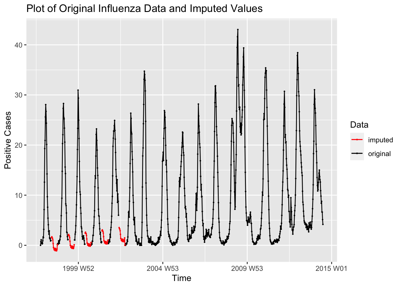
1.2 Time Plots
Once we have imported a time series and created a tsibble object, we are now able to plot it using ggplot2. One of the wonderful features of the set of packages included in fpp3 is that it is integrated into tidyverse, allowing us to use functions such as autoplot(data, variable). In the code chunk below, I use the autoplot function on the bev tsibble saved in the previous section.
autoplot(bev, dollars) +
  labs(title = "US Beverage Manufacturer Product Shipments, Unadjusted",
       x = "Time",
       y = "Dollars, in Millions")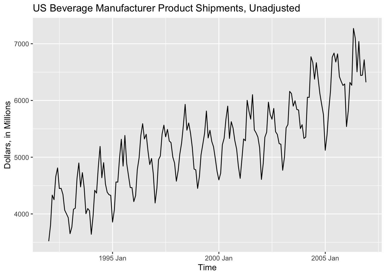
autoplot() is a wonderful function that can be used to quickly generate time series plots. It does a great job detecting the object type and generating an appropriate plot, but it is not a substitute for a tailored custom plot. Often it will be necessary to modify a plot or generate your own plot, as I did in the last one with the titles of the axes.
1.3 Seasonal Plots
Seasonal plots are graphics that are meant to better display the seasonality of data. fable offers two main functions to investigate the seasonality of the data: gg_season() and gg_subseries(). We will use the bev tsibble saved above as an example.
gg_season(data, y = ) is the standard included function for creating a seasonal plot. The output of this function is a modifyable ggplot object. In the code chunk below, I create a standard seasonal plot as seen in Forecasting: Principles and Practice.17 These plots use color to differentiate observations.
gg_season(bev, y = dollars) +
  labs(title = "US Beverage Manufacturer Product Shipments, Unadjusted",
       x = "Time",
       y = "Dollars, in Millions")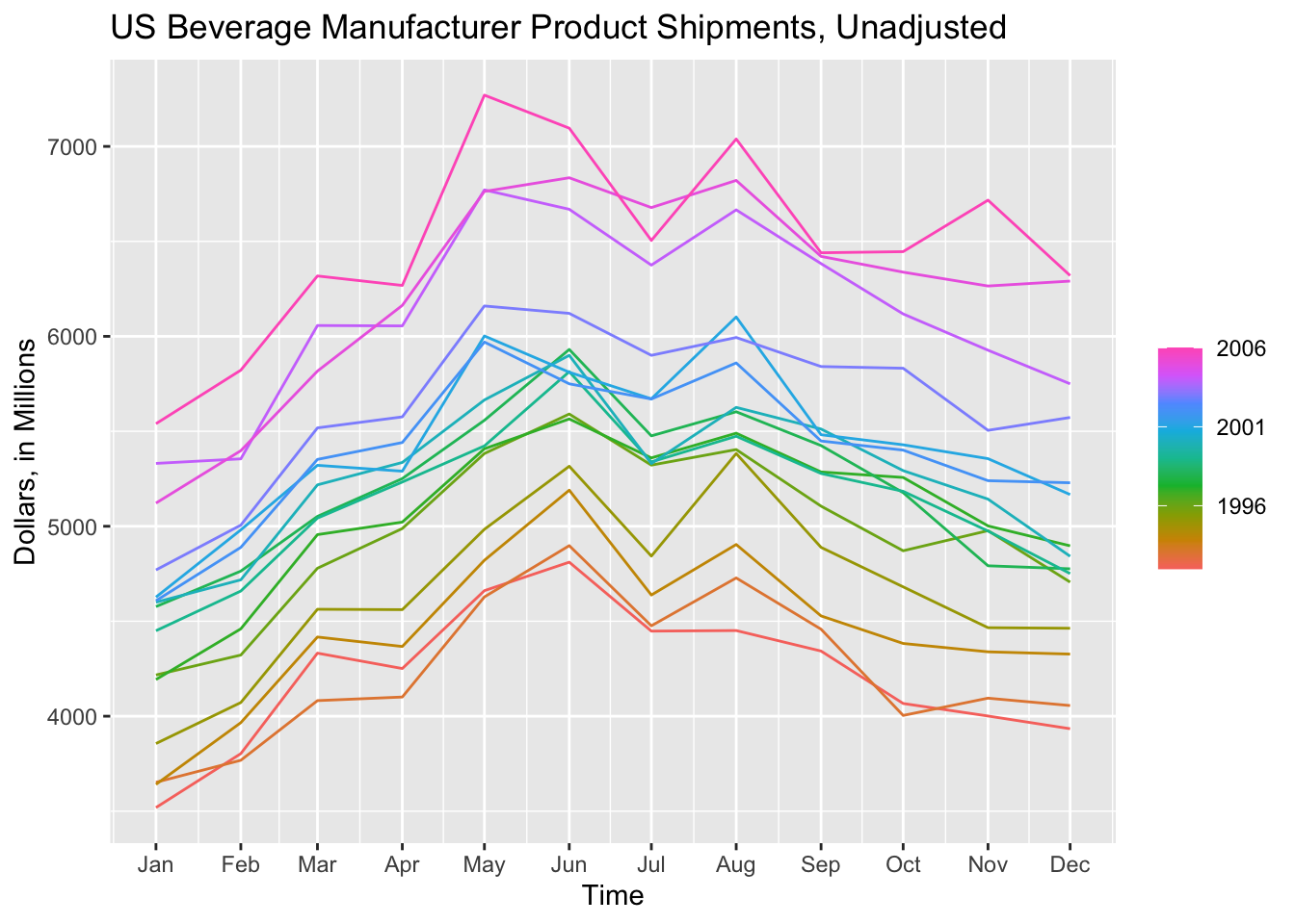
When examining a data set with fewer observations, such as bev, this produces a clear and interesting visualization. The label = parameter, demonstrated in the code chunk below, allows for the individual identification of each year.
gg_season(bev, y = dollars, labels = "right") +
  labs(title = "US Beverage Manufacturer Product Shipments, Unadjusted",
       x = "Time",
       y = "Dollars, in Millions")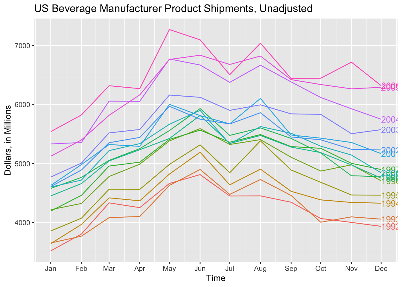
gg_subseries() creates a separate plot for each seasonal component, in this case month.18 The blue line indicates the mean for observations belonging to each month.
gg_subseries(bev, y = dollars) +
  labs(title = "US Beverage Manufacturer Product Shipments, Unadjusted",
       x = "Time",
       y = "Dollars, in Millions")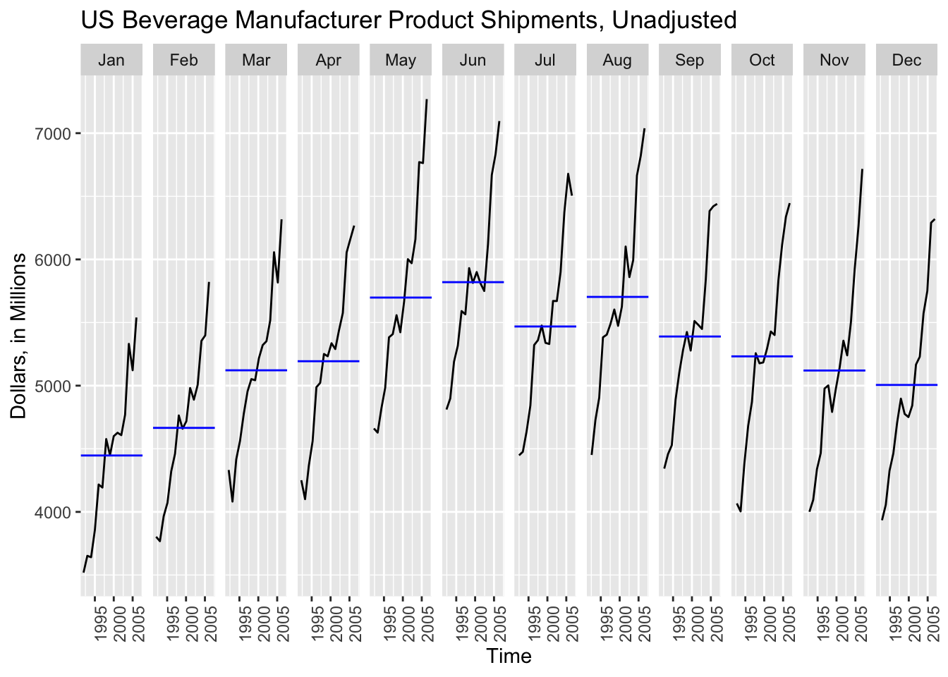
While gg_subseries() creates an interesting plot to observe the trend within a time category, such as month, the gg_season() plot easily becomes illegible when dealing with larger data sets and does not clearly indicate the year by using color.
I prefer to create my own seasonal plots using ggplot. In the plot below, I graph dollars on the y-axis and month on the x-axis using geom_point() and geom_line() and then facet wrap the whole plot by year. This creates a clear visualization that makes it easy to compare each year.
ggplot(bev, aes(x = month(time), y = dollars)) +
  geom_point(size = 0.25) +
  geom_line(linewidth = 0.25) +
  facet_wrap(~year(time)) +
  labs(title = "US Beverage Manufacturer Product Shipments, Unadjusted",
       x = "Month",
       y = "Dollars, in Millions")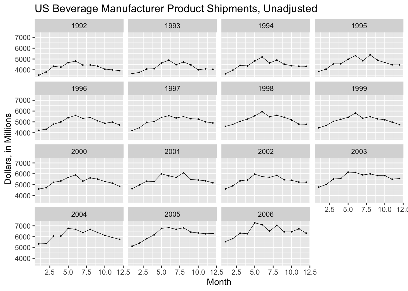
By graphing year along the x-axis and facet wrapping to month, I can create a similar plot to gg_subseries(), as shown below.
ggplot(bev, aes(x = year(time), y = dollars)) +
  geom_point(size = 0.25) +
  geom_line(linewidth = 0.25) +
  facet_wrap(~month(time)) +
  labs(title = "US Beverage Manufacturer Product Shipments, Unadjusted",
       x = "Year",
       y = "Dollars, in Millions")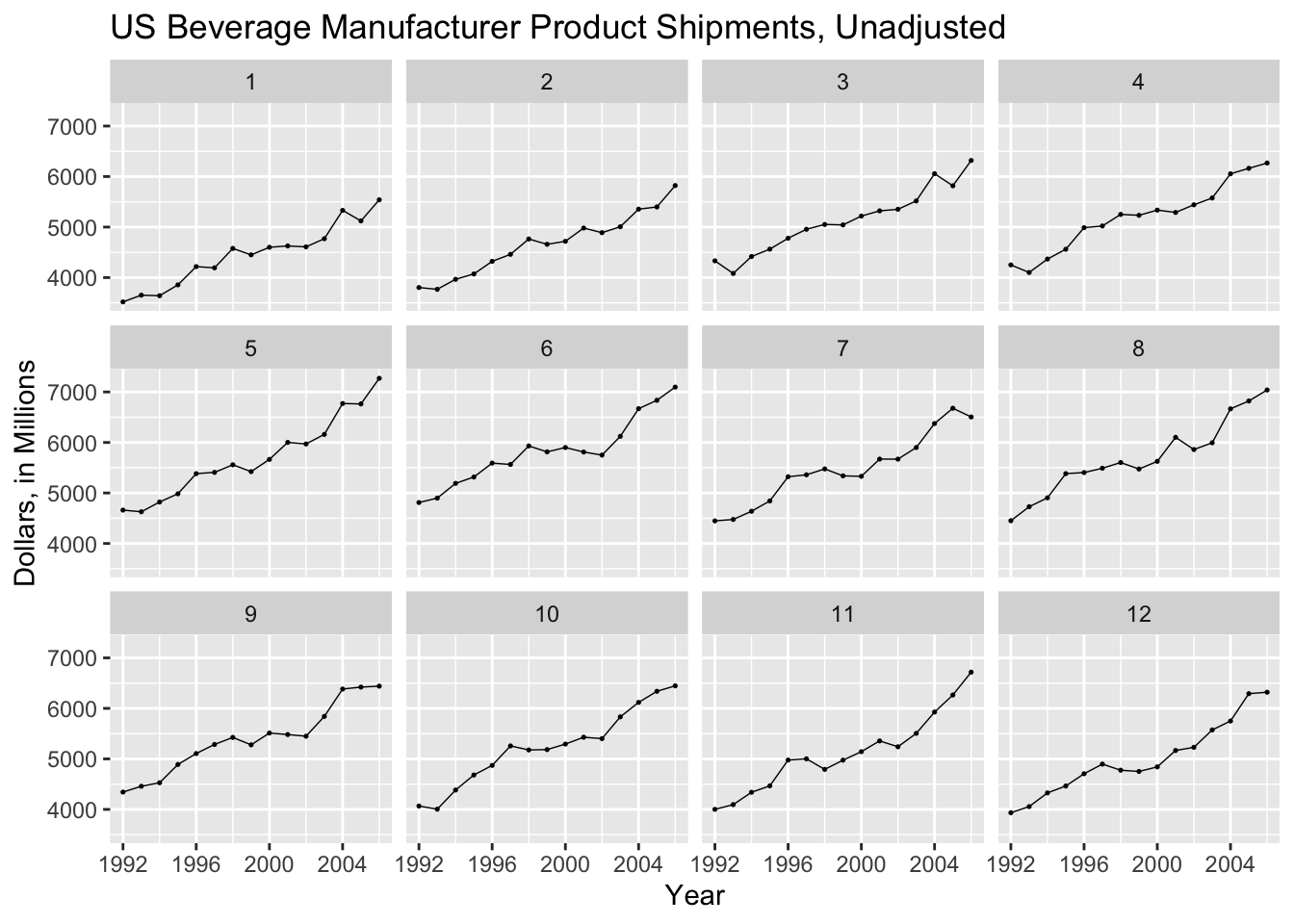
References
Montgomery, Jennings, and Kulahci, Introduction to Time Series Analysis and Forecasting.↩︎
Hyndman and Athanasopoulos, Forecasting Principles and Practice.↩︎
Montgomery, Jennings, and Kulahci, Introduction to Time Series Analysis and Forecasting.↩︎
Hyndman and Athanasopoulos, Forecasting Principles and Practice.↩︎
