3 Chapter 3: Regression Analysis and Forecasting

3.1 Introduction

Simple linear regression model: \(y = \beta_{0} + \beta_{1}x + \epsilon\)

Multiple linear regression model: \(y=\beta_{0}+\beta_{1}x_{1} + \beta_{2}x_{2} + ... +\beta_{k}x_{k} + \epsilon\)

Other examples: \(y = \beta_{0} + \beta_{1}x + \beta_{2}x^{2}+\epsilon\) \(y_{t} = \beta_{0}+\beta_{1} sin \frac{2 \pi}{d} t + \beta_{2} cos \frac{2 \pi}{d} t + \epsilon_{t}\)

Cross-section data: \(y_{i} = \beta_{0} + \beta_{1} x_{i1} + \beta_{2}x_{i2} + ... +\beta_{k}x_{ik} + \epsilon_{i}; \space i = 1,2,..,n\)

Time-series data: \(y_{t}=\beta_{0}+\beta_{1}x_{t_{1}}+\beta_{2}x_{t_{2}} + ... +\beta_{k}x_{t_{k}} + \epsilon_{t}, \space t=1,2,...,T\)

3.2 Least-Squares Estimation

Let \(\epsilon_{i} \sim D(0, \sigma^{2}); \space i = 1,2,...,n, \text{where } n \gt k\)

\[ \text{Least squares } f^{n}: L = \sum^{n}_{i=1} \epsilon_{i}^{2} \\ = \sum^{n}_{i=1}(y_{i}-\beta_{0}-\beta_{1}x_{i1}-\beta_{2}x_{i2}-...-\beta_{k}x_{ik})^{2} \\ = \sum^{n}_{i=1}(y_{i}-\beta_{0}-\sum_{j=1}^{k}\beta_{j}x_{ij})^{2} \]

For a minima of \(\{ \hat \beta_{j}\}_{j=0,1,...,k}\), FOC’s are: \[ \text{i.) } \frac{\delta L}{\delta \beta_{0}} \vert_{\beta_{1}, ..., \beta_{k}} = -2 \sum_{i=1}^{n}(y_{i}-\hat \beta_{0} - \sum_{j=1}^{k}\hat \beta_{j} x_{ij}) = 0 \\ \text{ii.) } \frac{\delta L}{\delta \beta_{j}} \vert_{\beta_{0}, \beta_{p \ne j}} = -2 \sum_{i=1}^{n}(y_{i}-\hat \beta_{0} - \sum_{j=1}^{k}\hat \beta_{j}) x_{ij} = 0 ; \space j = 1,2,...,k \]

Least Square Absurd Equation: Simplifying i.) and ii.), we have:

\[ n \hat \beta_{0} + \hat \beta_{1} \sum_{i=1}^{n}x_{i1} + \hat \beta_{2} \sum_{i=1}^{n} x_{i2} + ... +\hat \beta_{k} \sum_{i=1}^{n} x_{ik} = \sum_{i=1}^{n} y_{i} \\ \hat \beta_{0} \sum_{i=1}^{n} x_{i1} + \hat \beta_{1} \sum_{i=1}^{n} x_{i1}^{2} + \hat \beta_{2} \sum_{i=1}^{n} x_{i2}*x_{i1} + ... + \hat \beta_{k} \sum_{i=1}^{n} x_{ik}x_{i1} = \sum_{i=1}^{n} y_{i} x_{i1} \\ ... \\ \hat \beta_{0} \sum_{i=1}^{n} x_{ik} + \hat \beta_{1} \sum_{i=1}^{n} x_{i1}x_{ik} + \hat \beta_{2} \sum_{i=1}^{n} x_{i2} x_{ik} + ... + \hat \beta_{k} \sum_{i=1}^{n} x_{ik}^{2} = \sum_{i=1}^{n} y_{i} x_{ik} \]

Matrix form:

\[ y = X\beta+ \epsilon \text{, where} \\ y = \text{(n x 1) vector of obervations} \\ X = \text{(n x p) matrix of regrssors (model matrix)}\\ \beta = \text{(p x 1) vector of regression coefficients} \\ \epsilon = \text{(n x 1) vector of random errors}\\ L = \sum_{i=1}^{n} \epsilon_{i}^{2} = \epsilon \prime \epsilon = (y-X\beta)\prime (y-X\beta) \\ = y \prime y - \beta \prime X \prime y - y \prime X \beta + \beta \prime X \prime X \beta \\ = y \prime y - 2 \beta \prime X \prime y + \beta \prime X \prime X \beta \\ \text{Why? } \beta \prime X \prime y_{\text{(1 x 1)}} = y \prime X \beta_{\text{(1 x 1)}} \\ \frac{\delta L}{\delta \beta} \vert_{\hat \beta} = -2 X \prime y + 2 X \prime X \hat \beta = 0 \\ \to (X \prime X) \hat \beta = X \prime y \\ \therefore \hat \beta = (X \prime X)^{-1} X \prime y \]

Fitted values: \(\hat y = X \hat \beta\)

Residual: \(e = y - \hat y = y - X \hat \beta\)

\(\hat \sigma^{2} = \frac{SS_{E}}{n-k-1} = \frac{(y-X\hat \beta)\prime(y-X\hat \beta)}{n-k-1} = \frac{SS_{E}}{n-p}\)

If the model is “correct,” then \(\hat \beta\) is an unbiased estimator of the model parameters \(\beta\):

\(E(\hat \beta) = \beta\)

Also, \(var(\hat \beta) = \sigma^{2}(X \prime X)^{-1}\)

Example: trend adjustment

Fit a model with a linear time trend
Subtract the fitted values from original observations
Now, residuals are trend free
Forecast residuals
Add residual forecast value to estimate of trend, so
Now, we have a forecast of the variable

\(y_{t} - \beta_{0} + \beta_{1}t + \epsilon, \space t=1,2,...,T\)

Least squares normal equations for this model: \[ T \hat \beta_{0} + \hat \beta_{1} \frac{T(T+1)}{2} = \sum_{t=1}^{T} y_{t} \\ \hat \beta_{0} \frac{T(T+1)}{2} + \hat \beta_{1} \frac{T(T+1)(2T+1)}{6} = \sum_{t=1}^{T}t*y_{t} \\ \therefore \space \hat \beta_{0} = \frac{2(2T+1)}{T(T-1)} \sum_{t=1}^{T}y_{t} - \frac{6}{T(T-1)}\sum_{t=1}^{T} t*y_{t} \text{ , and} \\ \hat \beta_{1} = \frac{12}{T(T^{2}-1)} \sum_{t=1}^{T}t*y_{t} - \frac{6}{T(T-1)} \sum_{t=1}^{T} y_{t} \]

Procedure of previous page implies:

Let \(\hat \beta_{0}(T)\) and \(\hat \beta_{1}(T)\) denote the estimates of parameters completed at point in time T.
Predicting the next observation:
- a.) predict the point on the trend line in period T+1
  - \(\hat \beta_{0}(T) + \hat \beta_{1}(T)*(T+1)\)
- b.) add a forecast of the next residual
  - \(\hat e_{T+1}(1)\) - should be zero if structureless

\(\therefore \hat y_{T+1}(T) = \hat \beta_{0}(T) + \hat \beta_{1}(T)*(T+1)\)

3.3 Statistical Inference

hypothesis testing
confidence interval estimation
assume \(\epsilon_{i}\) (or \(\epsilon_{t}\)) \(\sim NID(0, \sigma^{2})\)

3.3.1 Test for significance of regression:

\[ H_{0}: \beta_{1} = \beta_{2} = ... =\beta_{k} = 0 \\ H_{1}: \text{at least one } \beta_{j} \ne 0 \\ SST = \sum_{i=1}^{n}(y_{i} - \bar y )^{2} = y \prime y - n \bar y^{2} \\ SSR = \hat \beta \prime X \prime y - n \bar y^{2} \\ SSE = y \prime y - \hat \beta \prime X \prime y \\ f_{0} = \frac{SSR / k}{SSE / (n-p)} \]

ANOVA Table

Source of Variation	Sum of Squares	D.F.	Mean Square	Test Stat
Regression	SSR	k	SSR/k	F = (SSR/k)/(SSE/(n-p))
Residual/Errors	SSE	n-p	SSE/(n-p)
Total	SST	n-1
Also see R-squared and adjusted-R-squared.

3.3.2 Tests for significance of individual regression coefficients

\[ H_{0}: \beta_{j} = 0 \\ H_{1}: \beta_{j} \ne 0 \\ t_{0} = \frac{\hat \beta_{j}}{se(\hat \beta_{j})} \\ \text{Reject } H_{0} \text{ if } \lvert t_{0} \rvert \gt t_{\frac{\alpha}{2}, n-p} \]

To test the significance of a group of coefficients, we can “partition” the model, and do a partial F-test.

\[ \text{Let } y = X \beta + \epsilon = X_{1} \beta_{1} + X_{2} \beta_{2} + \epsilon \\ \text{Then, } H_{0}: \beta_{1} = 0 \\ H_{1}: \beta_{1} \ne 0 \\ SSR(\beta_{1} \vert \beta_{2}) = SSR(\beta_{1}) - SSR(\beta_{2}) \\ = \hat \beta \prime X \prime y - \hat \beta_{2} \prime X_{2} \prime y \\ \therefore f_{0} = \frac{SSR(\beta_{1} \vert \beta_{2})/r}{\hat \sigma^{2}} \sim f(r, n-p) \]

3.3.3 Confidence Intervals on individual regression coefficients

If \(\epsilon \sim NID(0, \sigma^{2})\), then

\[ \hat \beta \sim N(\beta, \sigma^{2}(x\prime x)^{-1}) \]

Let \(C_{jj} = (jj)^{\text{th}}\) element of \((x \prime x)^{-1}\).

Then, a \((100 - \alpha)\)% confidence interval for \(\beta_{j}, \space j = 0,1,...,k\)

\(\lambda_{0}: \hat \beta_{j} - t_{\frac{\alpha}{2}, n-p}*\sqrt{\hat \sigma^{2} C_{jj}} \le \beta_{j} \le \hat \beta_{j} + t_{\frac{\alpha}{2}, n-p}* \sqrt{\hat \sigma^{2} C_{jj}}\)

\(\text{or: } \hat \beta_{j} - t_{\frac{\alpha}{2}, n-p}*se(\hat \beta_{j}) \le \beta_{j} \le \hat \beta_{j} + t_{\frac{\alpha}{2}, n-p} * se(\hat \beta_{j})\)

3.3.4 Confidence Interval on the Mean Response

Let \(x_{0} = \begin{bmatrix} 1 \\ x_{01} \\ ... \\ x_{0k} \end{bmatrix}\) be a particular combination of regressors.

Then, mean response at this point is: \[ E[y(x_{0})] = \mu_{y\vert x_{0}} = x_{0} \prime \beta, \text{ and} \\ \hat y(x_{0}) = \hat \mu_{y \vert x_{0}} = x_{0} \prime \hat p, \text{ and} \\ var(\hat y(x_{0})) = \hat \sigma^{2} x_{0}\prime (X \prime X)^{-1} x_{0} \]

Standard error of fitted response, \[ se(\hat y(x_{0})) = \sqrt{var(\hat y(x_{0}))} = \sqrt{\hat \sigma^{2} x_{0} \prime (X \prime X)^{-1}} x_{0} \\ \text{Then, a } (100-\alpha) \text{% confidence interval for mean response at } x_{0} \text{ is:} \\ \hat y(x_{0}) - t_{\frac{\alpha}{2}, n-p}*se(\hat y(x_{0})) \le \mu_{y \vert x_{0}} \le \hat y(x_{0}) + t_{\frac{\alpha}{2}, n-p}*se(\hat y(x_{0})) \]

3.3.5 Prediction of new observations

Let \(x_{0}\) be a particular set of values of regressors.

Point estimate of future observations, \(y(x_{0})\) is:

\(\hat y (x_{0}) = x_{0} \prime \hat p\)

Prediction error, \(e(x_{0}) = y(x_{0}) - \hat y(x_{0})\), and

\[ var(e(x_{0})) = var(y(x_{0}) - \hat y(x_{0})) \text{ assuming independence between } y \text{ and } \hat y \\ = var(y(x_{0})) + var(\hat y(x_{0})) \\ = \sigma^{2} + \sigma^{2} x_{0} \prime (X \prime X)^{-1} x_{0} \\ = \sigma^{2}(1 + x_{0} \prime (X \prime X)^{-1} x_{0}) \\ \therefore \text{s.e. of prediction error } = \sqrt{\hat \sigma^{2}(1+x_{0} \prime (X\prime X)^{-1}x_{0})} \sim t_{n-p} \\ \therefore \text{ A } (100 - \alpha) \text{ prediction interval for } y(x_{0}) \text{ is:} \\ \hat y (x_{0}) - t_{\frac{\alpha}{2}, n-p} \sqrt{\hat \sigma^{2}(1+x_{0} \prime (X \prime X)^{-1}x_{0}}) \le y(x_{0}) \le \hat y (x_{0}) + t_{\frac{\alpha}{2}, n-p} \sqrt{\hat \sigma^{2}(1+x_{0} \prime (X \prime X)^{-1}x_{0}}) \]

Confidence Interval: Interval estimate on MEAN RESPONSE of ‘\(y\)’ distribution at \(x_{0}\)

Prediction Interval: Interval estimate on a single future observation from the y distribution at \(x_{0}\)

3.3.6 Model Adequacy Checking:

Residual plots: \(e_{i} = y_{i} - \hat y_{i}; \space i = 1,2,...,n\)

assumption is \(\epsilon_{i} \sim NID(0, \sigma^{2})\)
Normal probability plot: normality of errors
Residuals vs fitted: constant variance/ equality of variance
residuals vs regressors
residuals vs time order: especially for time-series data

Standardize residuals: \(d_{i} = \frac{e_{i}}{\hat \sigma}; \space \hat \sigma^{2} =MSE\)

If \(\lvert d_{i} \rvert \gt 3\), examine the outliers

Studentized residuals: for heteroskedastic variance

\[ \hat y = X \hat \beta = X[(X \prime X)^{-1} X \prime y] \\ = (X(X \prime X)^{-1} X \prime)*y \\ = Hy; \space H = \text{hat matrix} \\ \therefore e = y - \hat y = y - Hy = y(I-H) \\ cov(e) = \sigma^{2}(I-H): \text{ covariance matrix} \\ v(e_{i}) = \sigma^{2}(1-h_{ii}) \\ \therefore \text{ Studentized Residuals: } r_{i} = \frac{e_{i}}{\sqrt{\hat \sigma^{2}(1-h_{ii})}} ; \hat \sigma ^{2} = MSE \]

Prediction error sum of squares (PRESS)

R-student: externally studentized residual

Cook’s distance: \(D_{i} = \frac{r_{i}^{2}}{p} * \frac{h_{ii}}{1-h_{ii}}\)

If \(D_{i} > 1 \to\) observation bias inference!
note: also see variable selection methods and model selection criteria. We will use ‘R’ to study this.

3.3.7 Generalized Least Squares, GLS

Problem: Heteroskedacity or non-constant variance

Solution(s): transform ‘\(y\)’ variable

\[ \text{Suppose } V= \begin{bmatrix} \sigma_{1}^{2} & 0 & ... & 0 \\ 0 & \sigma_{2}^{2} & 0 & 0 \\ ... & ... &... &... \\ 0 &0 & ...&\sigma_{n}^{2} \end{bmatrix} \text{, where} \\ \sigma_{i}^{2} = \text{variance of the i'th observation, } y_{i},\space i=1, 2, ..., n \]

We can create a “weighted least squares”(WLS) function, where the weight is inversely proportional to the variance of \(y_{i} \to w_{i} = \frac{1}{\sigma_{i}^{2}}\)

Then, \(L = \sum^{n}_{i=1} w_{i}(y_{i} - \beta_{0} - \beta_{1}x_{1})^{2}\), and the least squares normal equations are: \[ \hat \beta_{0} \sum_{i=1}^{n} w_{i} + \hat \beta_{1} \sum_{i=1}^{n} w_{i} x_{i} = \sum_{i=1}^{n} w_{i}y_{i} \\ \hat \beta_{0} \sum_{i=1}^{n} w_{i} x_{i} + \hat \beta_{1} \sum_{i=1}^{n} w_{i} x_{i}^{2} = \sum_{i=1}^{n}w_{i} x_{i} y_{i} \\ \text{Solve these to get } \hat \beta_{0} \text{ and } \hat \beta_{1} \]

In general, if \(y=X\beta + \epsilon, E(\epsilon) = 0;\) and \(var(\epsilon) = \sigma ^{2}V\) (not \(\sigma^{2} I\))

Then, the least squares function is: \(L = (y - X \beta)\prime V^{-1} (y-X\beta)\)

Least squares normal equations are: \((X\prime V^{-1}X) \hat \beta_{GLS} = X \prime V^{-1}y\)

GLS estimator of \(\beta\) is:

\(\hat \beta_{GLS} = (X\prime V^{-1} X)^{-1} X\prime V^{-1} y\), and

\(var(\hat \beta_{GLS}) = \sigma^{2}(X\prime V^{-1} X)^{-1}\).

Note: \(\hat \beta_{GLS}\) is BLUE of \(\beta\)

Question: How do we estimate the “weights”?

Steps in finding a “variance equation”:

Fit an OLS: \(y = X\beta + \epsilon\); obtain \(e\) (as residuals)
Use residual diagnostics to determine if \(\sigma^{2}_{i} = f(y)\) (residuals vs fitted plot) or \(\sigma_{i}^{2} = f(x)\) (residuals vs regressor plot)
Regress \(\sqrt{e}\) on either \(y\) or \(x_{i}\), whichever is appropriate. Obtain an equation for predicting the variance of each observation: \(\hat s^{2}_{i} = f(x)\) or \(\hat s^{2}_{i} = f(y)\)
Use fitted values from the estimated variance function to obtain weights: \(w_{i} = \frac{1}{\hat s^{2}_{i}}; \space 1,2,...,n\)
Use these weights as the diagonal elements of the \(V^{-1}\) matrix in the GLS procedure.
Iterate to reduce difference between \(\hat \beta_{OLS}\) and \(\hat \beta_{GLS}\)

Example: See R code for example

We can also use “discounted” least squares, where recent observations are weighted more heavily than older observations.

3.3.8 Regression models for general time-series data

If errors are correlated or not independent:

i.) \(\hat \beta_{OLS}\) is still unbiased, but not BLUE, i.e.; \(\hat \beta_{OLS}\) does not have minimum variance [SHOW … exercise] ii.) If errors are positively autocorrelated, MSE is (serious) underestimate of \(\sigma^{2}\)

standard error of \(\hat \beta\) are underestimated
confidence intervals and prediction intervals are shorter than they should be
\(H_{0}\) may be rejected more frequently than should be, and hypothesis tests are no longer reliable

Potential solutions to autocorrelated errors

If autocorrelation is due to an omitted variable, then identifying and including the appropriate omitted variable should remove the autocorrelation.
If we “understand” the structure of the autocorrelation, the use GLS.
Use models that specifically accounts for the autocorrelation

Consider a simple linear regression with “first-order” autoregressive errors, i.e.:

\(y_{t} = \beta_{0} + \beta_{1} x_{t} + \epsilon_{t}\), where

\(\epsilon_{t} = \phi \epsilon_{t-1} + a_{t}\), and \(a_{t} \sim NID(0, \sigma^{2}_{a})\), and \(\lvert \phi \rvert \lt 1\).

First, note that: \[ \epsilon_{t} = \phi \epsilon_{t-1} + a_{t} \\ = \phi(\phi \epsilon_{t-2} + a_{t-1}) + a_{t} \\ = \phi(\phi(\phi \epsilon_{t-3} + a_{t-2})+ a_{t-1}) + a_{t} \\ ... \\ \to \epsilon_{t} = \phi^{2} \epsilon_{t-2} + \phi a_{t-1} + a_{t} \\ = \phi^{3}\epsilon_{t-3} + \phi^{2} a_{t-2} + \phi a_{t-1} + a_{t} \\ = \phi^{3}\epsilon_{t-3} + \phi^{2} a_{t-2} + \phi^{1} a_{t-1} + \phi^{0} a_{t} \\ ... \\ \to \epsilon_{t} = \sum_{j=0}^{t} \phi^{j} a_{t-j} \\ \]

Also: [SHOW THESE DIY]

\[ a. \space E(\epsilon_{t}) = 0 \\ b. \space var(\epsilon_{t}) = \sigma^{2} = \sigma^{2}_{a}(\frac{1}{1-\phi^{2}}), \text{ and} \\ c. cov(\epsilon_{t}, \epsilon_{t \pm j}) = \phi^{j} \sigma_{a}^{2}(\frac{1}{1-\phi^{2}}) \]

Lag one autocorrelation, \(\rho_{1}\) is:

\[ \rho_{1} = \frac{cov(\epsilon_{t}, \epsilon_{t+1})}{\sqrt{var(\epsilon_{t})}* \sqrt{var(\epsilon_{t+1})}} = \phi \text{ (SHOW)} \]

Lag ‘k’ autocorrelation, \(\rho_{k}\) is:

\[ ACF: \rho_{k} = \frac{cov(\epsilon_{t}, \epsilon_{t+k})}{\sqrt{var(\epsilon_{t})}*\sqrt{var(\epsilon_{t+k})}} = \phi^{k} \]

3.3.8.1 Durbin-Watson Test for Autocorrelation

\[ \text{Positive autocorrelation: } H_{0}: \phi = 0; \space H_{1}: \phi \gt 1 \text{(correct)} \\ d = \frac{\sum_{t=2}^{T}(e_{t} - e_{t-1})^{2}}{\sum_{t=2}^{T} e^{2}_{t}} \approx 2(1-r_{1}) \\ \text{where } r_{1} = \text{lag one autocorrelation between residuals} \]

Positive Autocorrelation:

If \(d \lt d_{L}\): reject \(H_{0}: \phi = 0\)
If \(d \lt d_{u}\): do not reject \(H_{0}\)
If \(d_{L} \lt d \lt d_{u}\): inconclusive

Negative Autocorrelation:

If \((4-d) \lt d_{L}\): reject \(H_{0}\)
If \((4-d) \gt d_{L}\): do not reject \(H_{0}\)
IF \(d_{L} \lt 4-d \lt d_{u}\): inconclusive

3.3.8.2 Estimating Parameters in a Time Series Regression Model

Omission of one or more important predictor variables can cause ‘accidental’ time dependence. See example 3.13.

Cochran-Orcutt Method: Simple linear regression with AR(1) errors.

Let \(y_{t} = \beta_{0} + \beta_{1} x_{t} + \epsilon_{t}; \space \epsilon_{t} = \phi \epsilon_{t-1} + a_{t}\)

\(a_{t} \sim NID(0, \sigma^{2}_{a}); \space \lvert \phi \rvert \lt 1\)

Step 1: Transform \(y_{t}:\)

\[ \space y_{t} \prime = y_{t} - \phi y_{t-1} \\ \to y_{t}\prime = \beta_{0} + \beta_{1} x_{t} + \epsilon_{t} - \phi (\beta_{0} + \beta_{1} x_{t-1} + \epsilon_{t-1}) \\ \text{Note: } \beta_{0} + \beta_{1} x_{t} + \epsilon_{t} = y_{t} \text{ and } \beta_{0} + \beta_{1} x_{t-1} + \epsilon_{t-1} = y_{t-1} \\ \to y_{t} \prime = \beta_{0}(1-\phi) + \beta_{1}(x_{t}-\phi x_{t-1}) + (\epsilon_{t} - \phi \epsilon_{t-1}) \\ \text{Note: } \beta_{0} \prime = \beta_{0}(1-\phi), \space x_{t}\prime = x_{t}-\phi x_{t-1} \text{, and } a_{t} = \epsilon_{t} - \phi \epsilon_{t-1} \\ \to y_{t}\prime = \beta_{0} \prime + \beta_{1} x_{t} \prime + a_{t} \] Step 2: Get \(e_{t} : \space y_{t} - \hat y_{t}\)

Step 3: Estimate \(\phi: \space e_{t} = \hat \phi e_{t-1}\)

Recall: \(\hat \phi = \frac{\sum_{t=2}^{T} e_{t} e_{t-1}}{\sum_{t=1}^{T} e_{t}^{2}}\) (Recall: \(\frac{X\prime y}{X \prime X}\))

Step 4: Calculate \(y_{t} \prime = y_{t} - \hat \phi y_{t-1}\) and \(x_{t} \prime = x_{t} - \hat \phi x_{t-1}\)

Step 5: Estimate: \(\hat y_{t} \prime = \hat \beta_{0} \prime + \hat \beta_{1} x_{t} \prime\)

Step 6: Apply Durbin-Watson Test on \(a_{t} = y_{t} \prime - \hat y_{t} \prime\). If autocorrelation persists, REPEAT process! See example 3.14.

3.3.8.3 Maximum Likelihood Approach

Let \(y_{t} = \mu + a_{t}; \space a_{t} \sim N(0,\sigma^{2}); \space \mu = \text{unknown constant}\)

Probability density function of \(\{ y_{t} \}_{t=1,2,...,T}:\)

\[ f(y_{t}) = \frac{1}{\sqrt{2 \pi \sigma^{2}}} exp[\frac{1}{2} (\frac{y_{t}-\mu}{\sigma})^{2}] \\ \to f(y_{t}) = \frac{1}{\sqrt{2 \pi \sigma^{2}}} exp[- \frac{1}{2} (\frac{a_{t}}{\sigma})^{2}] \\ \]

Joint probability density function of \(\{ y_{1}, y_{2}, ..., y_{T} \}:\)

\[ l(y_{t}, \mu) = \prod_{t=1}^{T} f(y_{t}) = \prod_{t=1}^{T} \frac{1}{\sqrt{2 \pi \sigma^{2}}} exp[-\frac{1}{2} (\frac{a_{t}}{\sigma})^{2}] \\ \therefore \space l(y_{t}, \mu) = (\frac{1}{\sqrt{2 \pi \sigma^{2}}})^{T} exp[\frac{-1}{2\sigma^{2}} \sum_{t=1}^{T} a^{2}_{t}] \text{ (This is the likelihood function)}\\ \]

Log-likelihood function:

\[ ln(y_{t}, \mu) = - \frac{T}{2} *ln(2\pi) - T* ln(\sigma) - \frac{1}{2 \sigma^{2}} \sum_{t=1}^{T} a_{t}^{2} \\ \]

To maximize the log-likelihood, minimize \(\sum_{t=1}^{T} a_{t}^{2}\), i.e.;

\[ \text{Minimize }\sum_{1}^{T} a_{t}^{2} = \sum_{1}^{T}(y_{t}-\mu)^{2} \\ \text{This is the same as the LS estimators!!} \]

Now consider \(y_{t} = \beta_{0} + \beta_{1} x_{t} + \epsilon_{t}; \space \epsilon_{t} = \phi \epsilon_{t-1} + a_{t}; \space \lvert \phi \rvert \lt 1; \space a_{t} \sim N(0,\sigma_{a}^{2})\)

Then,

\[ y_{t} - \phi y_{t-1} = (1-\phi) \beta_{0} + \beta_{1}(x_{t} - \phi x_{t-1}) + a_{t} \text{ (as in Cochrane-Orcutt)} \\ \to y_{t} = \phi y_{t-1} + (1-\phi)\beta_{0} + \beta_{1}(x_{t}- \phi x_{t-1}) + a_{t} \]

The joint pdf of \(a_{t}\)’s is:

\[ f(a_2, a_3, ..., a_T) = \prod_{t=2}^{T} \frac{1}{\sqrt{2 \pi \sigma^{2}_{a}}} exp[- \frac{1}{2} (\frac{a_{t}}{\sigma_{a}})^{2}] \\ = [\frac{1}{\sqrt{2 \pi \sigma_{a}^{2}}}]^{T-1} exp[- \frac{1}{2 \sigma^{2}_{a}} \sum_{t=2}^{T} a_{t}^{2}] \\ \]

Likelihood function: \(l(y_{t}, \phi, \beta_{0}, \beta_{1}) =\)

\[ [\frac{1}{\sqrt{2 \pi \sigma_{a}^{2}}}]^{T-1}*exp[- \frac{1}{2 \sigma_{a}^{2}} \sum_{t=2}^{T}(y_{t}-(\phi y_{t-1} + (1-\phi)\beta_{0} + \beta_{1}(x_{t} - \phi x_{t-1}))^{2}] \]

Log-likelihood: \(ln(y_{t}, \phi, \beta_{0}, \beta_{1}) =\)

\[ - \frac{T-1}{2} ln(2 \pi) - (T-1) ln(\sigma_{a}) \\ - \frac{1}{2 \sigma_{a}^{2}} \sum_{t=2}^{T}[y_{t} - (\phi y_{t-1} + (1-\phi) \beta_{0} + \beta_{1}(x_{t} - \phi x_{t-1}))]^{2} \]

To maximize the log-likelihood, minimize last term or RHS which is just the SSE!

3.3.8.4 One-period ahead forecast:

A \((100 - \alpha)\)% PI for lead-one forecast is:

\[ \hat y_{T+1}(T) \pm z_{\frac{\alpha}{2}}*\hat \sigma_{a} \text{, where}\\ \hat y_{T+1}(T) = \hat \phi y_{T} + (1-\hat \phi) \hat \beta_{0} + \hat \beta_{1}(x_{T+1} - \hat \phi x_{T}) \]

3.3.8.5 Two-periods ahead forecast:

\[ \hat y_{T+2}(T) = \hat \phi y_{T+1} + (1-\hat \phi)\hat \beta_{0} + \hat \beta_{1}(x_{T+2} - \hat \phi x_{T+1}) \\ = \hat \phi [\hat \phi y_{T} + (1- \hat \phi) \hat \beta_{0} + \hat \beta_{1}(x_{T+1} - \hat \phi x_{T})] + (1-\hat \phi) \hat \beta_{0} + \hat \beta_{1}(x_{T+2} - \hat \phi x_{T+1}) \]

This is assuming, \(y_{T}\) and \(x_{T}\) are known; \(x_{T+1}\) and \(x_{T+2}\) are known; but \(a_{T+1}\) and \(a_{T+2}\) are not known yet (realized).

Two-step-ahead forecast error:

\[ y_{T+2} - \hat y_{T+2}(T) = a_{T+2} + \hat \phi a_{T+1} \\ var(a_{T+2} + \hat \phi a_{T+1}) = \hat \sigma_{a}^{2} + \hat \phi^{2} \hat \sigma^{2}_{a} \\ = (1+ \hat \phi^{2}) \hat \sigma_{a}^{2} \]

A \((100 - \alpha)\)% prediction interval for two-step-ahead forecast is:

\[ \hat y_{T+2}(T) \pm z_{\frac{\alpha}{2}}* (1+ \hat \phi^{2}) \hat \sigma_{a} \]

3.3.8.6 \(\tau\)-periods-ahead foreasts:

\[ \hat y_{T+\tau}(T) = \hat \phi \hat y_{T+\tau-1}(T) + (1-\hat \phi) \hat \beta_{0} + \hat \beta_{1}(x_{T+\tau} - \hat \phi x_{T+\tau-1}) \]

\(\tau\)-step-ahead forecast error:

\[ y_{T+\tau} - \hat y_{T+\tau}(T) = a_{T+\tau} + \phi a_{T+\tau-1} + ... + \phi^{\tau -1} a_{T+1} \\ var(y_{T+\tau} - \hat y_{T+\tau}(T)) = (1+\phi^{2} + \phi^{3} + ... + \phi^{2(\tau-1)})\sigma_{a}^{2} \\ = \frac{\sigma_{a}^{2}(1-\phi^{2 \tau})}{(1+\phi^{2})} \\ \therefore \text{ A } (100 - \alpha) \text{% prediction interval for the lead-} \tau \text{ forecast is:} \\ \hat y_{T+\tau}(T) \pm z_{\frac{\alpha}{2}} * (\frac{1-\hat \phi^{2 \tau}}{1- \hat \phi^{2}})^{1/2}* \hat \sigma_{a} \]

3.3.8.7 What if \(X_{T+\tau}\) is now known?

Use an unbiased forecast of \(x_{T+1}: \space \hat x_{T+1}\), and use for forecast of \(y_{T+1}(T)\), and to calculate variance of the forecast error: \(\frac{1-\phi^{2\tau}}{1+\phi^{2}} \sigma_{a}^{2} + \beta_{1}^{2} \sigma_{x}^{2}(\tau)\)! See equations 3.114 - 3.118.

3.4 Chapter 3 R-Code

In the code chunk below, I load the basic packages we have been using so far.

library(fpp3)
library(tidyverse)
library(gt)

3.4.1 Using Matrix Multiplication

Matrix multiplication is an important element in the math behind forecasting. Below, I will demonstrate how to perform these operations in R. The code chunk below demonstrates how to create a matrix.

cons <- matrix(1, nrow=25, ncol=1) # matrix with 1s in every entry, 25 rows, 1 column
# creates a constant matrix

# create three different columns
x1 <- c(55, 46, 30, 35, 59, 61, 74, 38, 27, 51, 53, 41, 37, 24, 42, 50, 58, 60, 62, 68, 70, 79, 63, 39, 49)
x2 <- c(50, 24, 46, 48, 58, 60, 65, 42, 42, 50, 38, 30, 31, 34, 30, 48, 61, 71, 62, 38, 41, 66, 31, 42, 40)
y <- c(68, 77, 96, 80, 43, 44, 26, 88, 75, 57, 56, 88, 88, 102, 88, 70, 52, 43, 46, 56, 59, 26, 52, 83, 75)

#binds these columns together
X <- cbind(cons, x1, x2)

To perform matrix multiplication use %*%. t() function transposes the matrix. The code below demonstrates how to perform matrix multiplication operations.

# if you put the command in parentheses it automatically shows the result, as seen below
(xtx <- t(X) %*% X) #Solve for X'X

##            x1    x2
##      25  1271  1148
## x1 1271 69881 60814
## x2 1148 60814 56790

(xtx_inv <- solve(t(X) %*% X)) #Solve for (X'X)^-1, use the solve function to find the inverse

##                            x1            x2
##     0.699946097 -0.0061280859 -0.0075869820
## x1 -0.006128086  0.0002638300 -0.0001586462
## x2 -0.007586982 -0.0001586462  0.0003408657

(xty <- t(X) %*% y) #Solve for (X'y)

##     [,1]
##     1638
## x1 76487
## x2 70426

(beta <- solve(t(X) %*% X) %*% t(X) %*% y) #Note the use of %*% to denote matrix multiplication

##           [,1]
##    143.4720118
## x1  -1.0310534
## x2  -0.5560378

# step by step to solve B = (X'X)^-1(X'y)

3.4.2 Linear Regression with ANOVA Tables

For this section we will be using the data introduced in the previous section. In the code chunk below, I bind the columns together, make them into a data frame, and appropriately name the variables. Note: I did not make the data into a tsibble because it is not time series data.

patsat <- as.data.frame(cbind(x1, x2, y)) |>
  rename(age = 1, severity = 2, satisfaction = 3)
patsat |> gt()

age	severity	satisfaction
55	50	68
46	24	77
30	46	96
35	48	80
59	58	43
61	60	44
74	65	26
38	42	88
27	42	75
51	50	57
53	38	56
41	30	88
37	31	88
24	34	102
42	30	88
50	48	70
58	61	52
60	71	43
62	62	46
68	38	56
70	41	59
79	66	26
63	31	52
39	42	83
49	40	75

The fable package is meant to only model time series data, so for the following regressions we use functions available through the stats package included in base R. The lm() function creates a linear model, with the formula inside written as dependent ~ independent + independent2. The summary() function provides a summary of the model, and the anova() function provides an Analysis of Variance Table for the model.

In the code chunk below, I run the linear model \(\text{satisfaction} = \hat \beta_{0} + \hat \beta_{1} \text{age} + \hat \beta_{2} \text{severity}\):

(sat1.fit <- lm(satisfaction ~ age + severity, data=patsat)) # run a linear model of satisfaction on age and severity

## 
## Call:
## lm(formula = satisfaction ~ age + severity, data = patsat)
## 
## Coefficients:
## (Intercept)          age     severity  
##     143.472       -1.031       -0.556

#same results as above using matrix algebra
summary(sat1.fit)

## 
## Call:
## lm(formula = satisfaction ~ age + severity, data = patsat)
## 
## Residuals:
##      Min       1Q   Median       3Q      Max 
## -17.2800  -5.0316   0.9276   4.2911  10.4993 
## 
## Coefficients:
##             Estimate Std. Error t value Pr(>|t|)    
## (Intercept) 143.4720     5.9548  24.093  < 2e-16 ***
## age          -1.0311     0.1156  -8.918 9.28e-09 ***
## severity     -0.5560     0.1314  -4.231 0.000343 ***
## ---
## Signif. codes:  0 '***' 0.001 '**' 0.01 '*' 0.05 '.' 0.1 ' ' 1
## 
## Residual standard error: 7.118 on 22 degrees of freedom
## Multiple R-squared:  0.8966, Adjusted R-squared:  0.8872 
## F-statistic: 95.38 on 2 and 22 DF,  p-value: 1.446e-11

anova(sat1.fit)

## Analysis of Variance Table
## 
## Response: satisfaction
##           Df Sum Sq Mean Sq F value    Pr(>F)    
## age        1 8756.7  8756.7 172.847 6.754e-12 ***
## severity   1  907.0   907.0  17.904 0.0003429 ***
## Residuals 22 1114.5    50.7                      
## ---
## Signif. codes:  0 '***' 0.001 '**' 0.01 '*' 0.05 '.' 0.1 ' ' 1

Next, I run the model \(\text{satisfaction} = \hat \beta_{0} + \hat \beta_{1} \text{age} + \hat \beta_{2} \text{severity} + \hat \beta_{3} \text{age}^{2}\). The first ANOVA table analyzes the variance between the variables in the model, when the second ANOVA table analyzes the variance between the models.

# add I to create an indicator variable, adds quadratic term
sat2.fit<-lm(satisfaction ~ age + severity + I(age^2), data=patsat)
summary(sat2.fit)

## 
## Call:
## lm(formula = satisfaction ~ age + severity + I(age^2), data = patsat)
## 
## Residuals:
##     Min      1Q  Median      3Q     Max 
## -16.931  -4.709   1.282   4.088  10.721 
## 
## Coefficients:
##               Estimate Std. Error t value Pr(>|t|)    
## (Intercept) 140.878301  16.992148   8.291 4.62e-08 ***
## age          -0.924787   0.660588  -1.400 0.176130    
## severity     -0.552431   0.136215  -4.056 0.000569 ***
## I(age^2)     -0.001064   0.006508  -0.164 0.871682    
## ---
## Signif. codes:  0 '***' 0.001 '**' 0.01 '*' 0.05 '.' 0.1 ' ' 1
## 
## Residual standard error: 7.281 on 21 degrees of freedom
## Multiple R-squared:  0.8967, Adjusted R-squared:  0.882 
## F-statistic: 60.78 on 3 and 21 DF,  p-value: 1.598e-10

anova(sat2.fit)

## Analysis of Variance Table
## 
## Response: satisfaction
##           Df Sum Sq Mean Sq  F value    Pr(>F)    
## age        1 8756.7  8756.7 165.2008 2.031e-11 ***
## severity   1  907.0   907.0  17.1119 0.0004686 ***
## I(age^2)   1    1.4     1.4   0.0267 0.8716819    
## Residuals 21 1113.1    53.0                       
## ---
## Signif. codes:  0 '***' 0.001 '**' 0.01 '*' 0.05 '.' 0.1 ' ' 1

anova(sat1.fit, sat2.fit)

## Analysis of Variance Table
## 
## Model 1: satisfaction ~ age + severity
## Model 2: satisfaction ~ age + severity + I(age^2)
##   Res.Df    RSS Df Sum of Sq      F Pr(>F)
## 1     22 1114.5                           
## 2     21 1113.1  1    1.4171 0.0267 0.8717

Next, I run the model \(\text{satisfaction} = \hat \beta_{0} + \hat \beta_{1} \text{age} + \hat \beta_{2} \text{severity} + \hat \beta_{3} \text{age}^{2} + \hat \beta_{4} \text{satisfaction}^{2}\)

# patient satisfaction is highly correlated with the severity of their condition, add quadratic severity term
sat3.fit<-lm(satisfaction ~ age + severity + I(age^2) + I(severity^2), data=patsat)
summary(sat3.fit)

## 
## Call:
## lm(formula = satisfaction ~ age + severity + I(age^2) + I(severity^2), 
##     data = patsat)
## 
## Residuals:
##     Min      1Q  Median      3Q     Max 
## -17.451  -3.485   2.234   3.794   9.087 
## 
## Coefficients:
##                 Estimate Std. Error t value Pr(>|t|)    
## (Intercept)    1.247e+02  2.638e+01   4.727 0.000129 ***
## age           -9.282e-01  6.662e-01  -1.393 0.178796    
## severity       1.659e-01  9.013e-01   0.184 0.855831    
## I(age^2)      -7.429e-04  6.575e-03  -0.113 0.911163    
## I(severity^2) -7.718e-03  9.570e-03  -0.806 0.429482    
## ---
## Signif. codes:  0 '***' 0.001 '**' 0.01 '*' 0.05 '.' 0.1 ' ' 1
## 
## Residual standard error: 7.342 on 20 degrees of freedom
## Multiple R-squared:    0.9,  Adjusted R-squared:   0.88 
## F-statistic: 44.99 on 4 and 20 DF,  p-value: 1.002e-09

#only intercept remains ss, model is statistically significant
anova(sat3.fit)

## Analysis of Variance Table
## 
## Response: satisfaction
##               Df Sum Sq Mean Sq  F value    Pr(>F)    
## age            1 8756.7  8756.7 162.4500 4.652e-11 ***
## severity       1  907.0   907.0  16.8270 0.0005541 ***
## I(age^2)       1    1.4     1.4   0.0263 0.8728218    
## I(severity^2)  1   35.1    35.1   0.6503 0.4294824    
## Residuals     20 1078.1    53.9                       
## ---
## Signif. codes:  0 '***' 0.001 '**' 0.01 '*' 0.05 '.' 0.1 ' ' 1

anova(sat1.fit, sat3.fit)

## Analysis of Variance Table
## 
## Model 1: satisfaction ~ age + severity
## Model 2: satisfaction ~ age + severity + I(age^2) + I(severity^2)
##   Res.Df    RSS Df Sum of Sq      F Pr(>F)
## 1     22 1114.5                           
## 2     20 1078.1  2    36.472 0.3383  0.717

Finally, the last linear model I run is \(\text{satisfaction} = \hat \beta_{0} \text{age} + \hat \beta_{1} \text{severity} + \hat \beta_{2} \text{age}*\text{satisfaction} + \hat \beta_{3} \text{age}^{2} + \hat \beta_{4} \text{satisfaction}^{2}\):

# model has age, severity, age*severity (interaction term), age^2, severity^2
sat4.fit<-lm(satisfaction ~ age + severity + age:severity + I(age^2)+ I(severity^2), data=patsat)
summary(sat4.fit)

## 
## Call:
## lm(formula = satisfaction ~ age + severity + age:severity + I(age^2) + 
##     I(severity^2), data = patsat)
## 
## Residuals:
##     Min      1Q  Median      3Q     Max 
## -16.915  -3.642   2.015   4.000   9.677 
## 
## Coefficients:
##                 Estimate Std. Error t value Pr(>|t|)    
## (Intercept)   127.527542  27.912923   4.569  0.00021 ***
## age            -0.995233   0.702072  -1.418  0.17251    
## severity        0.144126   0.922666   0.156  0.87752    
## I(age^2)       -0.002830   0.008588  -0.330  0.74534    
## I(severity^2)  -0.011368   0.013533  -0.840  0.41134    
## age:severity    0.006457   0.016546   0.390  0.70071    
## ---
## Signif. codes:  0 '***' 0.001 '**' 0.01 '*' 0.05 '.' 0.1 ' ' 1
## 
## Residual standard error: 7.503 on 19 degrees of freedom
## Multiple R-squared:  0.9008, Adjusted R-squared:  0.8747 
## F-statistic:  34.5 on 5 and 19 DF,  p-value: 6.76e-09

anova(sat4.fit)

## Analysis of Variance Table
## 
## Response: satisfaction
##               Df Sum Sq Mean Sq  F value    Pr(>F)    
## age            1 8756.7  8756.7 155.5644 1.346e-10 ***
## severity       1  907.0   907.0  16.1138 0.0007417 ***
## I(age^2)       1    1.4     1.4   0.0252 0.8756052    
## I(severity^2)  1   35.1    35.1   0.6228 0.4397609    
## age:severity   1    8.6     8.6   0.1523 0.7007070    
## Residuals     19 1069.5    56.3                       
## ---
## Signif. codes:  0 '***' 0.001 '**' 0.01 '*' 0.05 '.' 0.1 ' ' 1

3.4.3 Confidence and Prediction Interval Estimation

Next, I cover how to estimate confidence and prediction intervals for the models from the last section. confint(model, level = ) calculates the confidence intervals from the model object at the desired significance level.

#CIs for individual regression coefficients
confint(sat1.fit,level=.95) # 5% significance, 95% confidence interval

##                  2.5 %      97.5 %
## (Intercept) 131.122434 155.8215898
## age          -1.270816  -0.7912905
## severity     -0.828566  -0.2835096

confint(sat1.fit,level=.99) # 1% significance, 99% confidence interval

##                   0.5 %      99.5 %
## (Intercept) 126.6867763 160.2572473
## age          -1.3569331  -0.7051738
## severity     -0.9264513  -0.1856243

Next, I create new data and then use that new data to create a prediction interval. Notice the new data only contains age and severity but does not contain satisfaction. The predict(model, newdata =) function allows me to calculate a confidence and prediction interval for mean response. Note: this observation is in the sample.

#CIs and PIs for MEAN RESPONSE when observation is in sample
new1  <- data.frame(age=55, severity=50)
# predict adds new data and specifies that it is looking at a confidence interval
pred.sat1.ci.1<-predict(sat1.fit, newdata=new1, se.fit = TRUE, interval = "confidence")
pred.sat1.pi.1<-predict(sat1.fit, newdata=new1, se.fit = TRUE, interval = "prediction")
# only standard error is larger in prediction interval (it has the same mean so mean response will be the same), the interval size is larger for the prediction interval

pred.sat1.ci.1$fit

##        fit      lwr      upr
## 1 58.96218 55.83594 62.08843

pred.sat1.pi.1$fit

##        fit      lwr      upr
## 1 58.96218 43.87363 74.05074

Finally, I create a confidence and prediction interval for new data outside of the sample using the same functions as the example above:

#CIs and PIs for MEAN RESPONSE when observation is NOT in sample
new2 <- data.frame(age=60, severity=60)
pred.sat1.ci.2<-predict(sat1.fit, newdata=new2, se.fit = TRUE, interval = "confidence")
pred.sat1.pi.2<-predict(sat1.fit, newdata=new2, se.fit = TRUE, interval = "prediction")

pred.sat1.ci.2$fit

##        fit      lwr      upr
## 1 48.24654 43.84806 52.64501

pred.sat1.pi.2$fit

##        fit      lwr      upr
## 1 48.24654 32.84401 63.64906

Finally, I create a confidence and prediction interval for a future observation.

#CIs and PIs for future observations
new3 <- data.frame(age=75, severity=60)
pred.sat1.ci.3<-predict(sat1.fit, newdata=new3, se.fit = TRUE, interval = "confidence")
pred.sat1.pi.3<-predict(sat1.fit, newdata=new3, se.fit = TRUE, interval = "prediction")

pred.sat1.ci.3$fit

##        fit      lwr      upr
## 1 32.78074 26.99482 38.56666

pred.sat1.pi.3$fit

##        fit      lwr      upr
## 1 32.78074 16.92615 48.63533

3.4.4 Calculating Prediction Values Step by Step

Now, I will demonstrate how to calculate these intervals in R step by step. This is often a good exercise in understanding the math behind these measures.

First, I create variables containing the number of rows (observations) and columns (variables).

(nrow <- dim(patsat)[1])

## [1] 25

(ncol <- dim(patsat)[2])

## [1] 3

Next, I calculate the \(\sigma^{2}\) and the RMSE. The t() function transposes the matrix parameter.

(sig.sq <- (t(y)%*%y - t(sat1.fit$coefficients)%*%t(X)%*%y)/(nrow-ncol)) #calculates sigma squared

##          [,1]
## [1,] 50.66118

(se_hat <- sqrt(sig.sq)) #This is equation 3.34; also the RMSE in Table 3.3

##          [,1]
## [1,] 7.117667

Next, I calculate the predicted value of y when given new data:

x0 <- c(1, 75, 60) #Age=75; Severity=60
pred.y.x0 <- t(x0) %*% sat1.fit$coefficients

Then, I calculate the standard error of the fit and the prediction, as well as the t-statistic at 95% CI:

(se.fit <- sqrt(sig.sq * (t(x0)%*% xtx_inv %*% x0))) #See SE(Fit) in table 3.6

##         [,1]
## [1,] 2.78991

(se.pred.err <- sqrt(sig.sq * (1 + (t(x0)%*% xtx_inv %*% x0)))) #See SE(Pred) in Table 3.6

##          [,1]
## [1,] 7.644918

#t-statistic at 95% CI and relevant degrees of freedom
(tval <- qt((1-0.95)/2, df=nrow-ncol))

## [1] -2.073873

Finally, after calculating all necessary values, I calculate the confidence interval for the mean response and the prediction interval for future observations:

# Confidence interval for mean response
(ci.y.xo.lwr <- pred.y.x0 - tval*se.fit) #CIs of mean response - Lower limit

##          [,1]
## [1,] 38.56666

(ci.y.xo.upr <- pred.y.x0 + tval*se.fit) #CIs of mean response - Upper limit

##          [,1]
## [1,] 26.99482

#Prediction interval for future observation
(pi.y.xo.lwr <- pred.y.x0 - tval*se.pred.err) #CIs of mean response - Lower limit

##          [,1]
## [1,] 48.63533

(pi.y.xo.upr <- pred.y.x0 + tval*se.pred.err) #CIs of mean response - Upper limit

##          [,1]
## [1,] 16.92615

3.4.5 Model Adequacy Checks

The first thing to look at when checking the adequacy of a model are the residuals. Below, I define the residual plotting function introduced in the last chapter.

# required packages
library(tidyverse)
library(fpp3)
library(qqplotr)
library(gridExtra)
# custom function:
plot_residuals <- function(df, title = ""){
    df <- df |>
    mutate(scaled_res = scale(.resid) |> as.vector())
  
  lb_test <- df |> features(.resid, ljung_box)
  print(lb_test)
  
  print(ACF(df, y = .resid, na.action = na.omit) |> autoplot() + labs(title = paste("AFC of", title)))
  
  plot1 <- df |>
    ggplot(aes(sample = scaled_res)) + 
    geom_qq(size = 0.25, na.rm = TRUE) + 
    stat_qq_line(linewidth = 0.25, na.rm = TRUE) + 
    stat_qq_band(alpha = 0.3, color = "red", na.rm = TRUE) + 
    labs(x = "Sample Quantile", y = "Residual")
  
  plot2 <- df |>
    ggplot(mapping = aes(x = .resid)) + 
    geom_histogram(aes(y = after_stat(density)), na.rm = TRUE, bins = 20) + 
    stat_function(fun = dnorm, args = list(mean = mean(df$.resid), sd = sd(df$.resid)), color = "red", na.rm = TRUE) +
    labs(y = "Frequency", x = "Residual")
  
  plot3 <- df |>
    ggplot(mapping = aes(x = .fitted, y = .resid)) + 
    geom_point(size = 0.25, na.rm = TRUE) + 
    geom_line(linewidth = 0.25, na.rm = TRUE) + 
    labs(x = "Fitted Value", y = "Residual")
  
  plot4 <- df |>
    ggplot(mapping = aes(x = time, y = .resid)) + 
    geom_point(size = 0.25, na.rm = TRUE) + 
    geom_line(linewidth = 0.25, na.rm = TRUE) + 
    labs(x = "Time", y = "Residual")
  
return(grid.arrange(plot1, plot3, plot2, plot4, top = paste(title, "Residual Plots")))
}
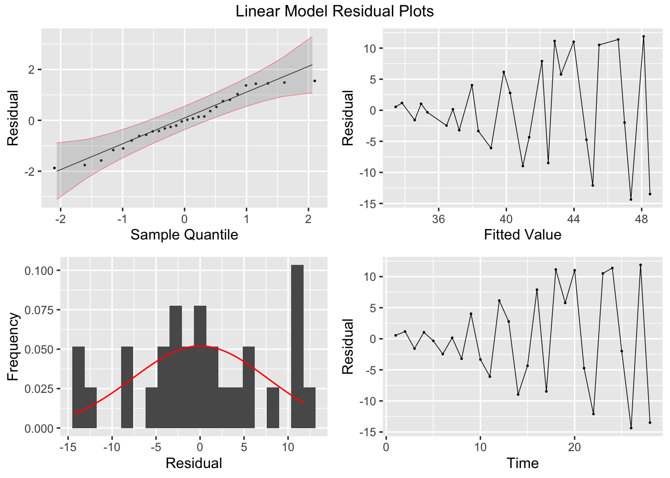
# to use this function you must have this code chunk in your document

The plot_residuals() function is mean to handle models that have been augmented in fable, so it cannot be used. Below, I create a tibble containing the information from the model needed for the residual plots and then create the residual plots for it outside of the function using similar code.

residuals <- tibble(.resid = sat1.fit$res,
                    .fitted = sat1.fit$fit) |>
  mutate(time = row_number(),
         scaled_res = scale(.resid) |> as.vector())

plot1 <- residuals |>
  ggplot(aes(sample = scaled_res)) + 
  geom_qq(size = 0.25, na.rm = TRUE) + 
  stat_qq_line(linewidth = 0.25, na.rm = TRUE) + 
  stat_qq_band(alpha = 0.3, color = "red", na.rm = TRUE) + 
  labs(x = "Sample Quantile", y = "Residual")
  
plot2 <- residuals |>
  ggplot(mapping = aes(x = .resid)) + 
  geom_histogram(aes(y = after_stat(density)), na.rm = TRUE, bins = 20) + 
  stat_function(fun = dnorm, args = list(mean = mean(residuals$.resid), sd = sd(residuals$.resid)), color = "red", na.rm = TRUE) +
  labs(y = "Frequency", x = "Residual")
  
plot3 <- residuals |>
  ggplot(mapping = aes(x = .fitted, y = .resid)) + 
  geom_point(size = 0.25, na.rm = TRUE) + 
  geom_line(linewidth = 0.25, na.rm = TRUE) + 
  labs(x = "Fitted Value", y = "Residual")
  
plot4 <- residuals |>
  ggplot(mapping = aes(x = time, y = .resid)) + 
  geom_point(size = 0.25, na.rm = TRUE) + 
  geom_line(linewidth = 0.25, na.rm = TRUE) + 
  labs(x = "Time", y = "Residual")

grid.arrange(plot1, plot3, plot2, plot4)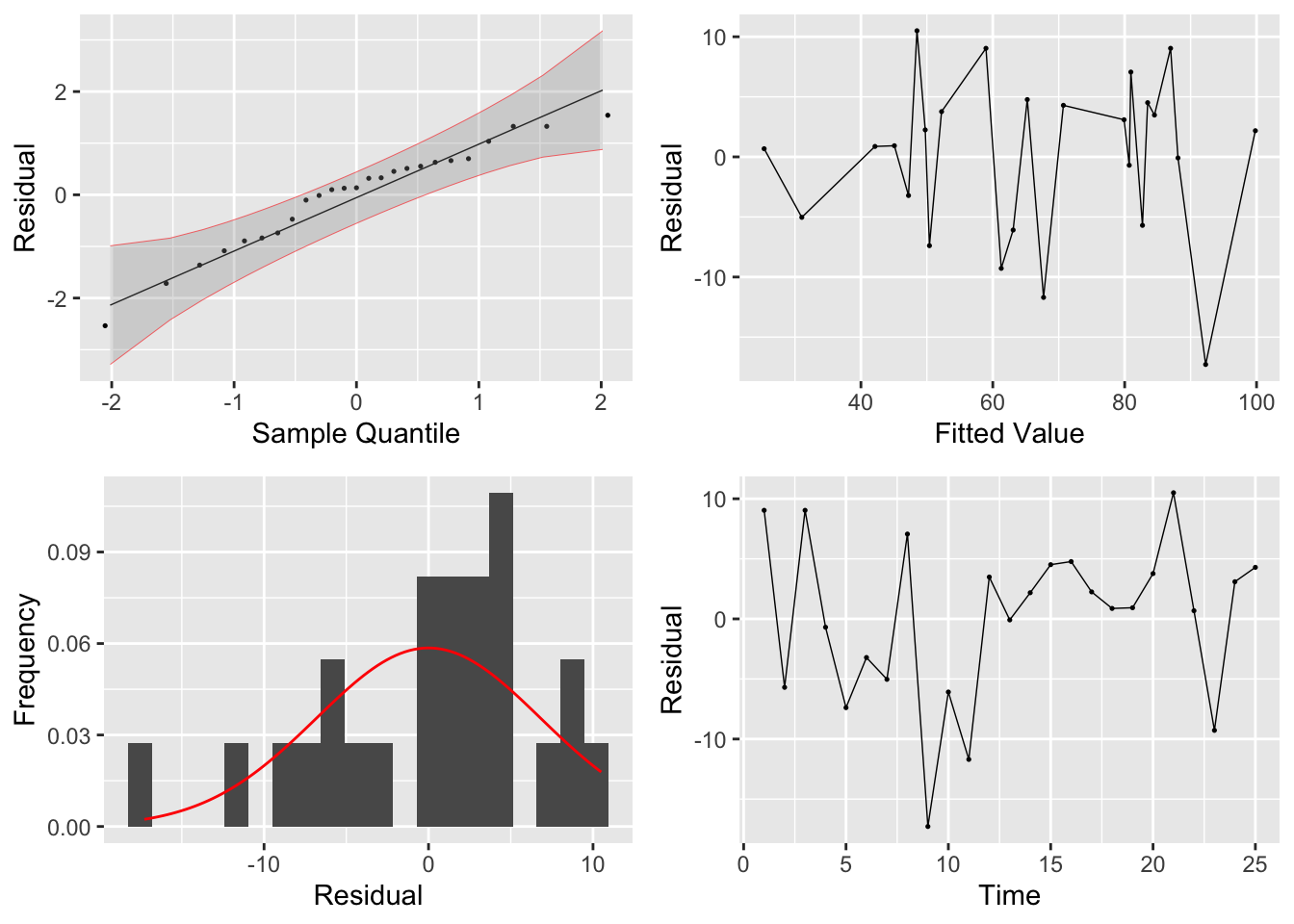

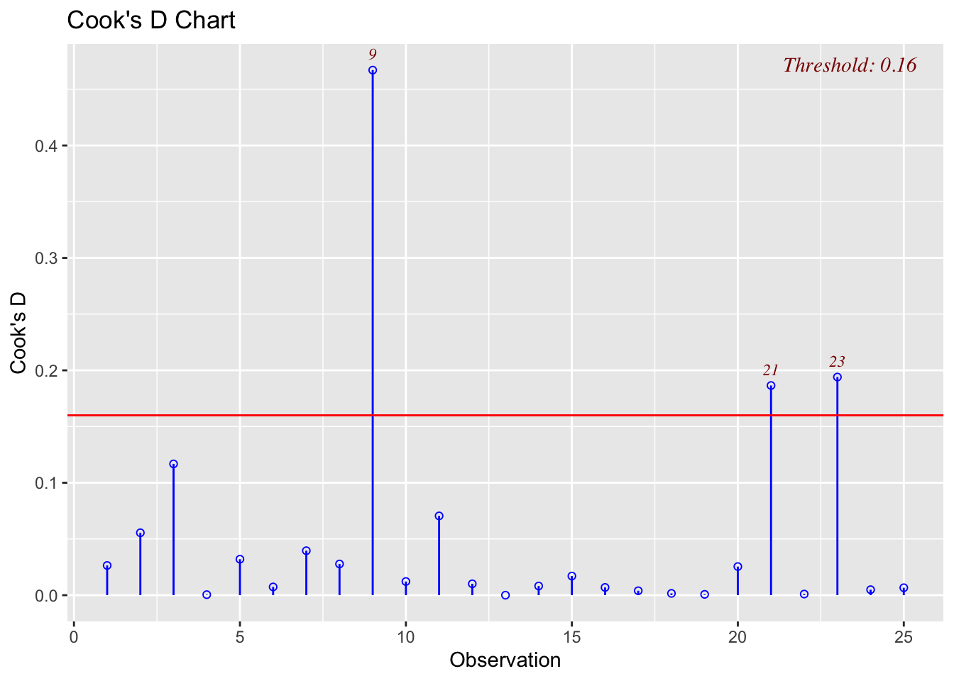
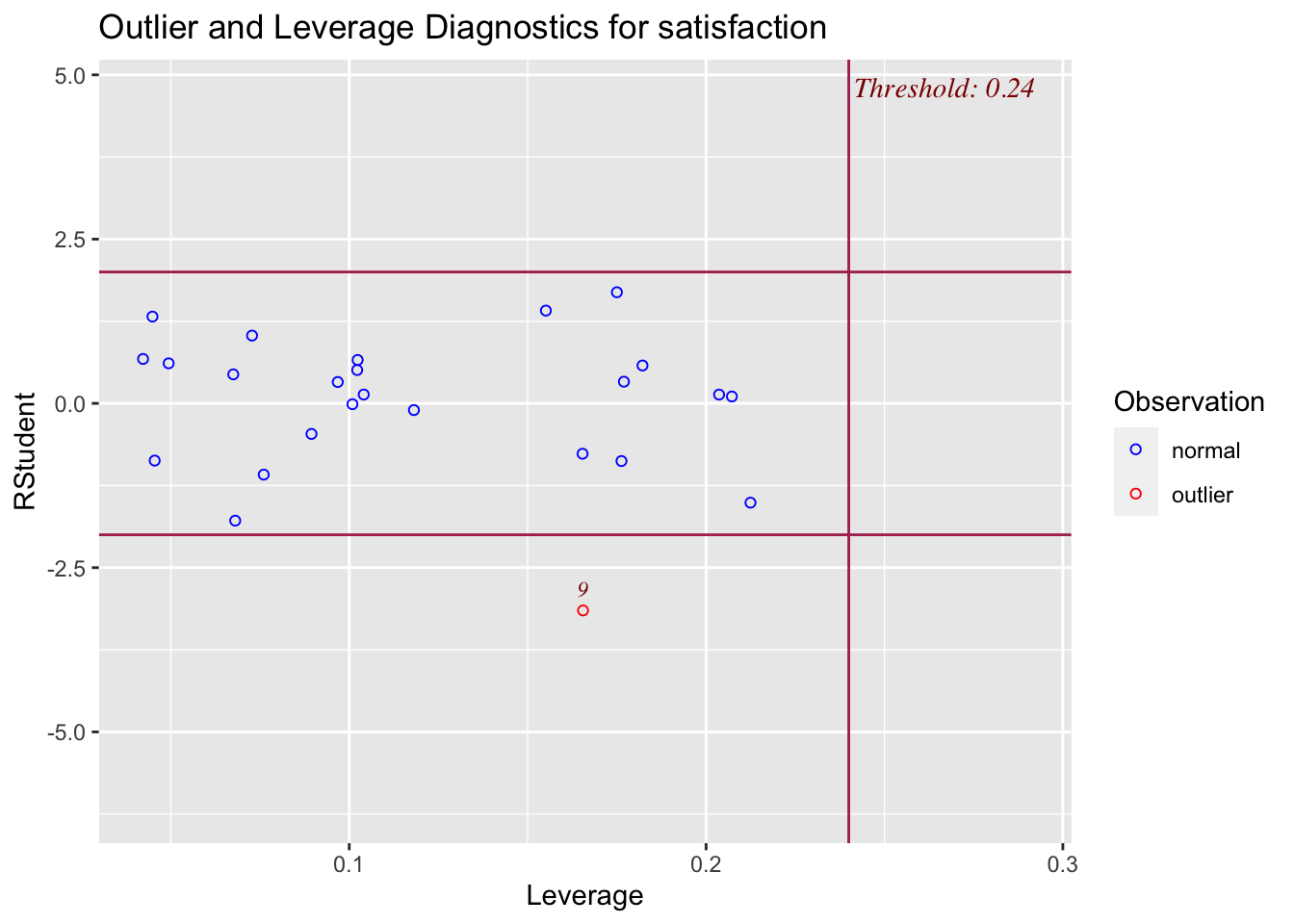
There are three other plots that can be used in model adequacy checks:

Studentized residual plots
Cook’s distance chart
Influential observation graph

The functions to produce these graphs are included in the olsrr package, called at the top of the code chunk below.

library(olsrr)

## 
## Attaching package: 'olsrr'

## The following object is masked from 'package:datasets':
## 
##     rivers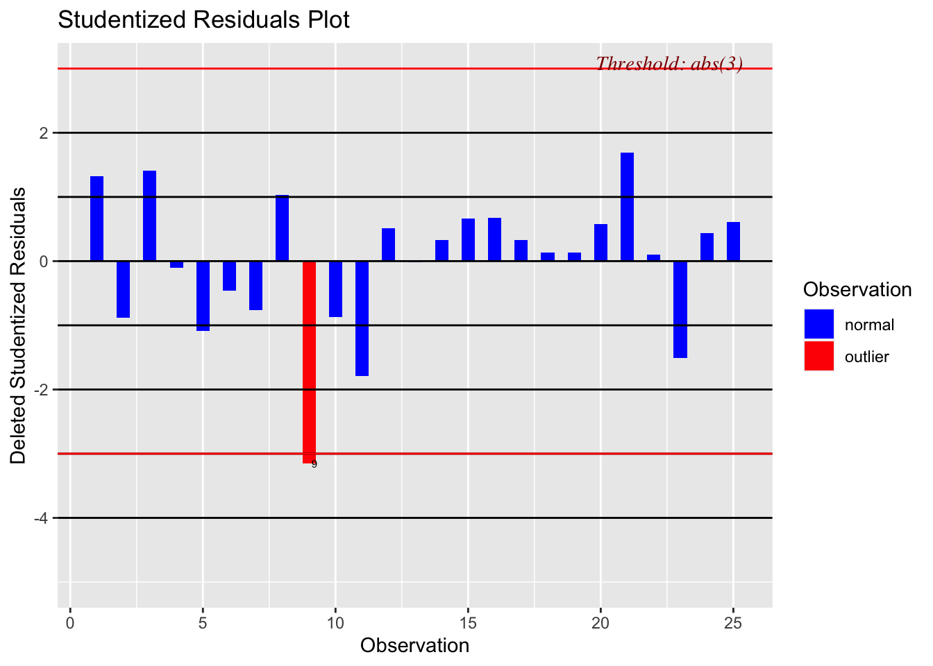

ols_plot_resid_stud(sat1.fit)   #Studentized residual plot

ols_plot_cooksd_chart(sat1.fit) #Cook's Distance chart

ols_plot_resid_lev(sat1.fit)    #Graph for detecting influential observations

#shows both values that have influence and outliers

A useful measure for evaluating model adequacy is Prediction Error Sum of Squares (PRESS). The function for this is included in the MPV package. This is demonstrated in the code chunk below:

library(MPV)

## Loading required package: lattice

## Loading required package: KernSmooth

## KernSmooth 2.23 loaded
## Copyright M. P. Wand 1997-2009

## Loading required package: randomForest

## randomForest 4.7-1.1

## Type rfNews() to see new features/changes/bug fixes.

## 
## Attaching package: 'randomForest'

## The following object is masked from 'package:gridExtra':
## 
##     combine

## The following object is masked from 'package:dplyr':
## 
##     combine

## The following object is masked from 'package:ggplot2':
## 
##     margin

## 
## Attaching package: 'MPV'

## The following object is masked from 'package:olsrr':
## 
##     cement

PRESS(sat1.fit)

## [1] 1484.934

3.4.6 Variable Selection Methods

First, we must add new variables to the existing data for this section. This is done in the code chunk below by creating vectors containing the new variables and them using the mutate() function to modify the existing data.

# automated nature and depends on the order that you put the variables
x3 <- c(0, 1, 1, 1, 0, 0, 1, 1, 0, 1, 1, 0, 0, 0, 0, 1, 1, 1, 0, 0, 1, 1, 1, 0, 1)
x4 <- c(2.1, 2.8, 3.3, 4.5, 2.0, 5.1, 5.5, 3.2, 3.1, 2.4, 2.2, 2.1, 1.9, 3.1, 3.0, 4.2, 4.6, 5.3, 7.2, 7.8, 7.0, 6.2, 4.1, 3.5, 2.1)

patsat <- patsat |> mutate(surg.med = x3, 
                           anxiety = x4)

Then, I run a linear model containing all variables with the equation: \(\text{satisfaction} = \hat \beta_{0} \text{age} + \hat \beta_{1} \text{severity} + \hat \beta_{2}\text{surg.med} + \hat \beta_{3} \text{anxiety}\)

(sat4.fit  <- lm(satisfaction ~ age + severity + surg.med + anxiety, data=patsat))

## 
## Call:
## lm(formula = satisfaction ~ age + severity + surg.med + anxiety, 
##     data = patsat)
## 
## Coefficients:
## (Intercept)          age     severity     surg.med      anxiety  
##    143.8672      -1.1172      -0.5862       0.4149       1.3064

Next, I run a forward selection algorithm that starts small and keeps adding variables.

(step.for  <- step(sat4.fit, direction='forward')) #forward selection algorithm, starts small and keeps adding variables

## Start:  AIC=103.18
## satisfaction ~ age + severity + surg.med + anxiety

## 
## Call:
## lm(formula = satisfaction ~ age + severity + surg.med + anxiety, 
##     data = patsat)
## 
## Coefficients:
## (Intercept)          age     severity     surg.med      anxiety  
##    143.8672      -1.1172      -0.5862       0.4149       1.3064

Then, I run a backwards selection algorithm, which starts with all the variables and compares the models resulting from subtracting variables.

(step.back <- step(sat4.fit, direction='backward')) #backward selection algorithm, starts large and keeps removing variables

## Start:  AIC=103.18
## satisfaction ~ age + severity + surg.med + anxiety
## 
##            Df Sum of Sq    RSS    AIC
## - surg.med  1       1.0 1039.9 101.20
## - anxiety   1      75.4 1114.4 102.93
## <none>                  1038.9 103.18
## - severity  1     971.5 2010.4 117.68
## - age       1    3387.7 4426.6 137.41
## 
## Step:  AIC=101.2
## satisfaction ~ age + severity + anxiety
## 
##            Df Sum of Sq    RSS    AIC
## - anxiety   1      74.6 1114.5 100.93
## <none>                  1039.9 101.20
## - severity  1     971.8 2011.8 115.70
## - age       1    3492.7 4532.6 136.00
## 
## Step:  AIC=100.93
## satisfaction ~ age + severity
## 
##            Df Sum of Sq    RSS    AIC
## <none>                  1114.5 100.93
## - severity  1     907.0 2021.6 113.82
## - age       1    4029.4 5143.9 137.17

## 
## Call:
## lm(formula = satisfaction ~ age + severity, data = patsat)
## 
## Coefficients:
## (Intercept)          age     severity  
##     143.472       -1.031       -0.556

The step.both() function compares conclusions from both methods and chooses the best fit.

step.both <- step(sat4.fit, direction='both') #compares both methods and chooses the best fit

## Start:  AIC=103.18
## satisfaction ~ age + severity + surg.med + anxiety
## 
##            Df Sum of Sq    RSS    AIC
## - surg.med  1       1.0 1039.9 101.20
## - anxiety   1      75.4 1114.4 102.93
## <none>                  1038.9 103.18
## - severity  1     971.5 2010.4 117.68
## - age       1    3387.7 4426.6 137.41
## 
## Step:  AIC=101.2
## satisfaction ~ age + severity + anxiety
## 
##            Df Sum of Sq    RSS    AIC
## - anxiety   1      74.6 1114.5 100.93
## <none>                  1039.9 101.20
## + surg.med  1       1.0 1038.9 103.18
## - severity  1     971.8 2011.8 115.70
## - age       1    3492.7 4532.6 136.00
## 
## Step:  AIC=100.93
## satisfaction ~ age + severity
## 
##            Df Sum of Sq    RSS    AIC
## <none>                  1114.5 100.93
## + anxiety   1      74.6 1039.9 101.20
## + surg.med  1       0.2 1114.4 102.93
## - severity  1     907.0 2021.6 113.82
## - age       1    4029.4 5143.9 137.17

This algorithm chooses the “best” model based on which one has the lowest AIC. This is not the only measure of whether a model is good.

library(leaps)
step.best<-regsubsets(satisfaction ~ age + severity + surg.med + anxiety, data=patsat)
summary(step.best)

## Subset selection object
## Call: regsubsets.formula(satisfaction ~ age + severity + surg.med + 
##     anxiety, data = patsat)
## 4 Variables  (and intercept)
##          Forced in Forced out
## age          FALSE      FALSE
## severity     FALSE      FALSE
## surg.med     FALSE      FALSE
## anxiety      FALSE      FALSE
## 1 subsets of each size up to 4
## Selection Algorithm: exhaustive
##          age severity surg.med anxiety
## 1  ( 1 ) "*" " "      " "      " "    
## 2  ( 1 ) "*" "*"      " "      " "    
## 3  ( 1 ) "*" "*"      " "      "*"    
## 4  ( 1 ) "*" "*"      "*"      "*"

# AIC is not a way to compare models objectively, theory has an important role

3.4.7 Generalized Least Squares

For this next example, I will use the data contained in ConnectorStregnth.csv.³⁰ In the code chunk below, I read in the data and use it to create a tsibble.

(cs_data <- read.csv("data/ConnectorStrength.csv") |> 
   as_tsibble(index = Observation) |>
   rename(time = 1, weeks = 2, strength = 3))

## # A tsibble: 28 x 3 [1]
##     time weeks strength
##    <int> <int>    <int>
##  1     1    20       34
##  2     2    21       35
##  3     3    23       33
##  4     4    24       36
##  5     5    25       35
##  6     6    28       34
##  7     7    29       37
##  8     8    30       34
##  9     9    32       42
## 10    10    33       35
## # ℹ 18 more rows

Next I create a simple linear model, regressing weeks on strength.

cs_data.fit <- cs_data |>
  model(TSLM(strength ~ weeks))

cs_data.fit |> report()

## Series: strength 
## Model: TSLM 
## 
## Residuals:
##       Min        1Q    Median        3Q       Max 
## -14.36394  -4.44492  -0.08607   5.86712  11.88420 
## 
## Coefficients:
##             Estimate Std. Error t value Pr(>|t|)    
## (Intercept)  25.9360     5.1116   5.074 2.76e-05 ***
## weeks         0.3759     0.1221   3.078  0.00486 ** 
## ---
## Signif. codes:  0 '***' 0.001 '**' 0.01 '*' 0.05 '.' 0.1 ' ' 1
## 
## Residual standard error: 7.814 on 26 degrees of freedom
## Multiple R-squared: 0.2671,  Adjusted R-squared: 0.2389
## F-statistic: 9.476 on 1 and 26 DF, p-value: 0.0048627

augment(cs_data.fit) |> 
  rename(`original` = strength, fitted = .fitted) |> 
  pivot_longer(c(`original`, fitted), names_to = "data") |>
  ggplot(aes(x = time, y = value, color = data)) +
  geom_point(size = 0.5) + 
  geom_line() + 
  labs(y = "strength", title = "Original Data vs Linear model of Strength on Weeks")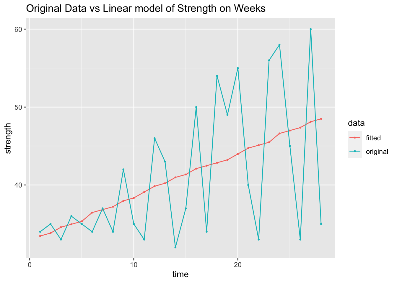

plot_residuals(augment(cs_data.fit), title = "Linear Model")

## # A tibble: 1 × 3
##   .model                 lb_stat lb_pvalue
##   <chr>                    <dbl>     <dbl>
## 1 TSLM(strength ~ weeks)    2.09     0.149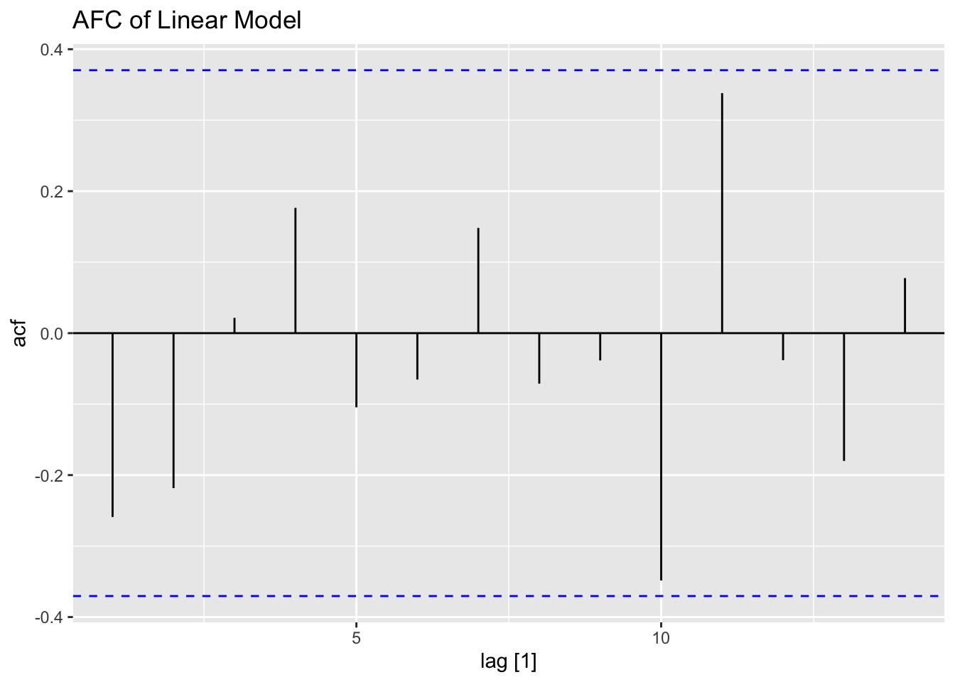

In addition to the normal residual plots, I create a plot with the original strength value on the x-axis and the residual of that observation on the x-axis.

augment(cs_data.fit) |> 
  mutate(orig = .fitted + .resid) |>
  ggplot(aes(x = orig, y = .resid)) +
  geom_point(size = 0.5) +
  geom_line() +
  labs(title = "Plot of Strength Data vs. Model Residuals", x = "Strength", y = "Residuals")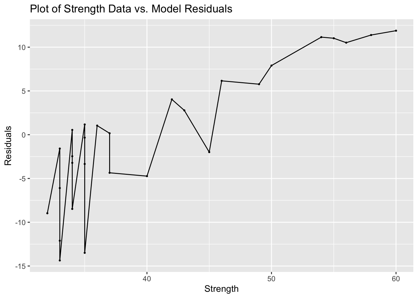

Next, I take the absolute value of the residuals and regress it on the x variable(weeks). I then calculate the weights for GLS using the formula \(\text{weight} = \frac{1}{\hat e ^{2}}\) and combine them with the original data.

resid_model <- cs_data |>
  left_join(augment(cs_data.fit) |> select(time, .resid), by = join_by(time)) |>
  mutate(abs.resid = abs(.resid)) |>
  model(TSLM(abs.resid ~ weeks))

cs_data.fit <- cs_data |> left_join(augment(resid_model) |> rename(resid_fit = .fitted) |> select(time, resid_fit), by = join_by(time)) |>
  mutate(weights = 1/(resid_fit^2))
cs_data.fit

## # A tsibble: 28 x 5 [1]
##     time weeks strength resid_fit weights
##    <int> <int>    <int>     <dbl>   <dbl>
##  1     1    20       34     0.116 73.9   
##  2     2    21       35     0.415  5.81  
##  3     3    23       33     1.01   0.977 
##  4     4    24       36     1.31   0.582 
##  5     5    25       35     1.61   0.386 
##  6     6    28       34     2.50   0.159 
##  7     7    29       37     2.80   0.127 
##  8     8    30       34     3.10   0.104 
##  9     9    32       42     3.70   0.0731
## 10    10    33       35     4.00   0.0626
## # ℹ 18 more rows

Then, I use the lm(formula, weights = , data = ) function to run the same regression but with the calculated weights. The resulting model retains statistical significance, but the magnitude has diminished.

gls_model <- lm(strength ~ weeks, weights = weights, data = cs_data.fit)
summary(gls_model)

## 
## Call:
## lm(formula = strength ~ weeks, data = cs_data.fit, weights = weights)
## 
## Weighted Residuals:
##     Min      1Q  Median      3Q     Max 
## -1.9695 -1.0450 -0.1231  1.1507  1.5785 
## 
## Coefficients:
##             Estimate Std. Error t value Pr(>|t|)    
## (Intercept) 27.54467    1.38051  19.953  < 2e-16 ***
## weeks        0.32383    0.06769   4.784 5.94e-05 ***
## ---
## Signif. codes:  0 '***' 0.001 '**' 0.01 '*' 0.05 '.' 0.1 ' ' 1
## 
## Residual standard error: 1.119 on 26 degrees of freedom
## Multiple R-squared:  0.4682, Adjusted R-squared:  0.4477 
## F-statistic: 22.89 on 1 and 26 DF,  p-value: 5.942e-05

3.4.8 Durbin-Watson Test for Autocorrelation

For this section, we will use the data from SoftDrinks.csv, which contains yearly observations on soft drink sales, expenditures, and population. Below, I read in the data and create a tsibble object.

(soft_drinks <- read_csv("data/SoftDrinks.csv") |> 
  rename(time = 1, sales = 2, exp = 3, pop = 4) |> 
  as_tsibble(index = time))

## Rows: 20 Columns: 4
## ── Column specification ───────────────────────────────────────
## Delimiter: ","
## dbl (4): Year, Sales, Expenditures, Population
## 
## ℹ Use `spec()` to retrieve the full column specification for this data.
## ℹ Specify the column types or set `show_col_types = FALSE` to quiet this message.

## # A tsibble: 20 x 4 [1]
##     time sales   exp    pop
##    <dbl> <dbl> <dbl>  <dbl>
##  1     1  3083    75 825000
##  2     2  3149    78 830445
##  3     3  3218    80 838750
##  4     4  3239    82 842940
##  5     5  3295    84 846315
##  6     6  3374    88 852240
##  7     7  3475    93 860760
##  8     8  3569    97 865925
##  9     9  3597    99 871640
## 10    10  3725   104 877745
## 11    11  3794   109 886520
## 12    12  3959   115 894500
## 13    13  4043   120 900400
## 14    14  4194   127 904005
## 15    15  4318   135 908525
## 16    16  4493   144 912160
## 17    17  4683   153 917630
## 18    18  4850   161 922220
## 19    19  5005   170 925910
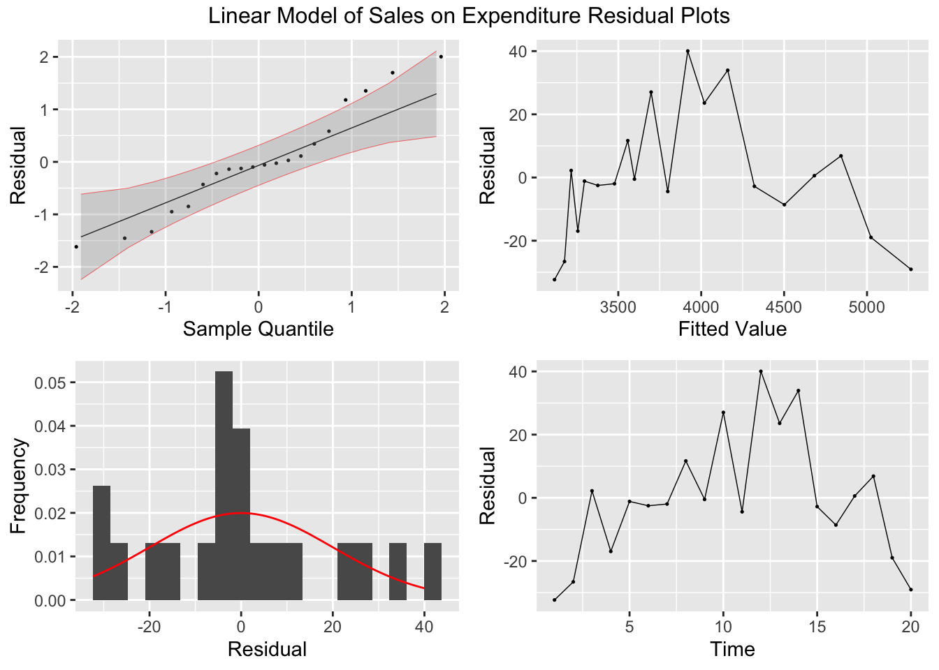
## 20    20  5236   182 929610

First, I run a simple linear regression of sales on expenditure and another linear model of sales on expenditure plus population, generate a report of the models, and run the plot_residuals() function.

soft_drinks.fit <- soft_drinks |>
  model(simple  = TSLM(sales ~ exp),
        exp_pop = TSLM(sales ~ exp + pop))

soft_drinks.fit |> select(simple) |> report()

## Series: sales 
## Model: TSLM 
## 
## Residuals:
##     Min      1Q  Median      3Q     Max 
## -32.330 -10.696  -1.558   8.053  40.032 
## 
## Coefficients:
##              Estimate Std. Error t value Pr(>|t|)    
## (Intercept) 1608.5078    17.0223   94.49   <2e-16 ***
## exp           20.0910     0.1428  140.71   <2e-16 ***
## ---
## Signif. codes:  0 '***' 0.001 '**' 0.01 '*' 0.05 '.' 0.1 ' ' 1
## 
## Residual standard error: 20.53 on 18 degrees of freedom
## Multiple R-squared: 0.9991,  Adjusted R-squared: 0.999
## F-statistic: 1.98e+04 on 1 and 18 DF, p-value: < 2.22e-16

plot_residuals(augment(soft_drinks.fit) |> filter(.model == "simple"), title = "Linear Model of Sales on Expenditure")

## # A tibble: 1 × 3
##   .model lb_stat lb_pvalue
##   <chr>    <dbl>     <dbl>
## 1 simple    2.61     0.106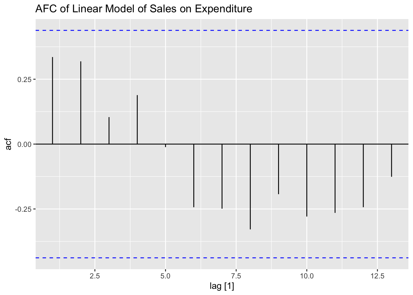

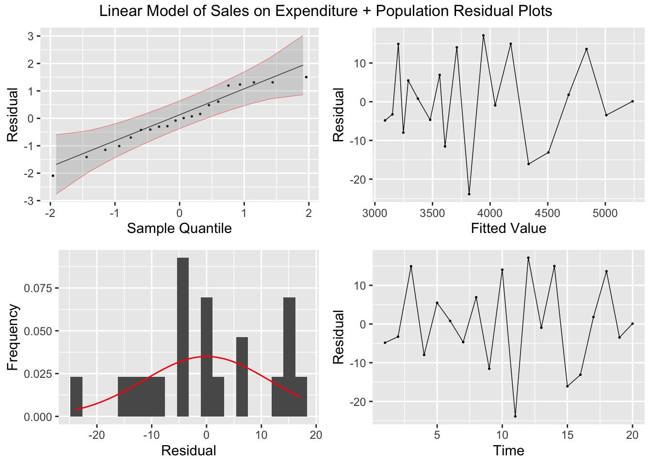
soft_drinks.fit |> select(exp_pop) |> report()

## Series: sales 
## Model: TSLM 
## 
## Residuals:
##      Min       1Q   Median       3Q      Max 
## -23.8654  -5.6178  -0.4197   8.5950  17.1334 
## 
## Coefficients:
##              Estimate Std. Error t value Pr(>|t|)    
## (Intercept) 3.203e+02  2.173e+02   1.474    0.159    
## exp         1.843e+01  2.915e-01  63.232  < 2e-16 ***
## pop         1.679e-03  2.829e-04   5.934 1.63e-05 ***
## ---
## Signif. codes:  0 '***' 0.001 '**' 0.01 '*' 0.05 '.' 0.1 ' ' 1
## 
## Residual standard error: 12.06 on 17 degrees of freedom
## Multiple R-squared: 0.9997,  Adjusted R-squared: 0.9997
## F-statistic: 2.873e+04 on 2 and 17 DF, p-value: < 2.22e-16

plot_residuals(augment(soft_drinks.fit) |> filter(.model == "exp_pop"), title = "Linear Model of Sales on Expenditure + Population")

## # A tibble: 1 × 3
##   .model  lb_stat lb_pvalue
##   <chr>     <dbl>     <dbl>
## 1 exp_pop    6.61    0.0101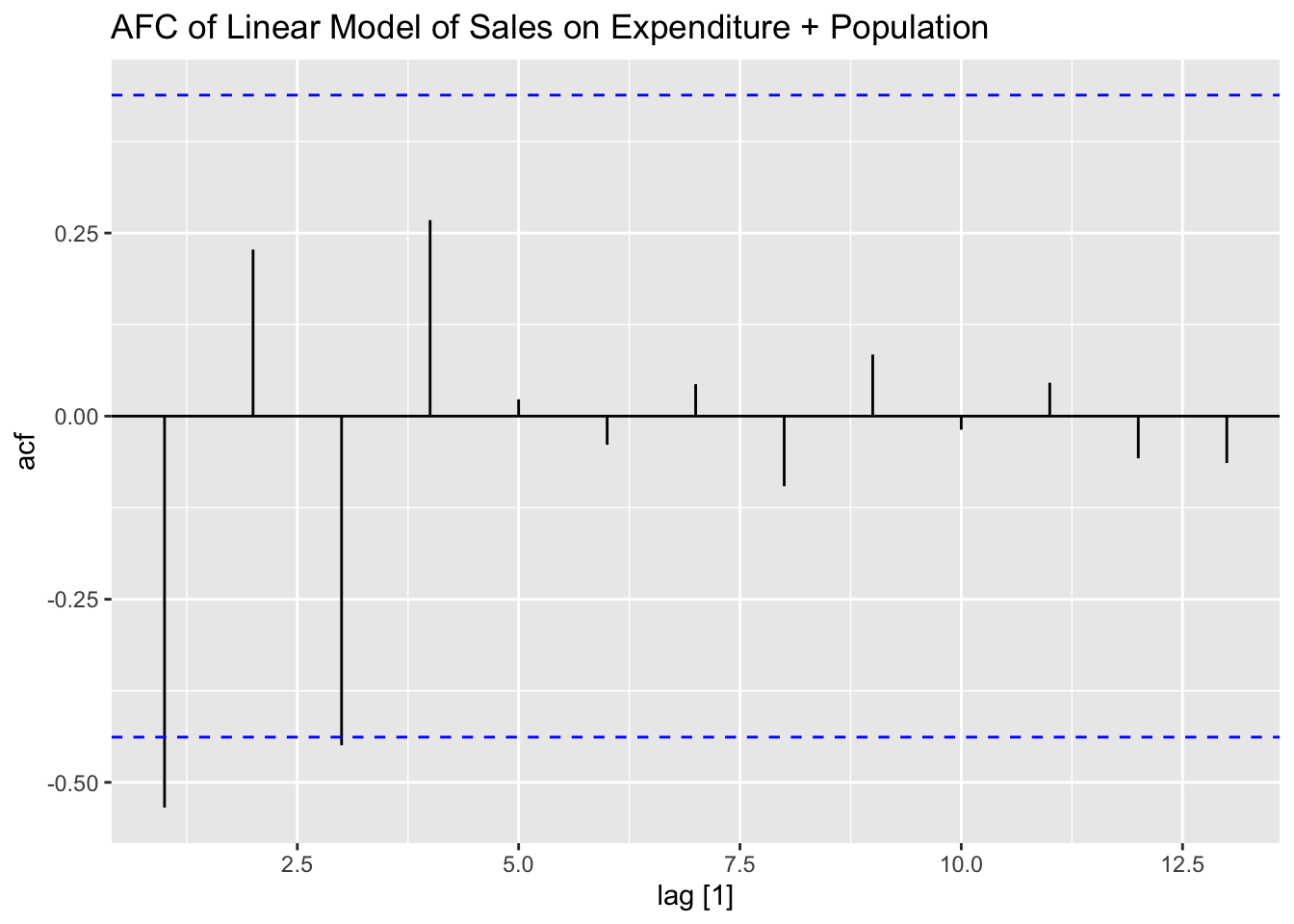

The formula for the Durbin-Watson test statistic is:

\[ d = \frac{\sum_{t=2}^{T}(e_{t}-e_{t-1})^{2}}{\sum_{t=1}^{T}e_{t}^{2}} = \frac{\sum_{t=2}^{T}e_{t}^{2} + \sum_{t=2}^{T}e_{t-1}^{2} - 2 \sum_{t=2}^{T}e_{t}e_{t-1}}{\sum_{t=1}^{T}e_{t}^{2}} \approx 2(1-r_{1}) \\ e_{t}, \space t = 1,2,...,T = \text{residuals from an OLS regression of } y_{t} \text{ on } x_{t} \\ r_{1} = \text{the lag one autocorrelation between the residuals} \]³¹

The dwt(model) function, included in the car package, accepts a vector of residuals as the model = parameter. This function returns the Durbin-Watson test statistic. In the code chunk below, I run the Durbin-Watson Test on both models.

library(car)

## Loading required package: carData

## 
## Attaching package: 'car'

## The following object is masked from 'package:dplyr':
## 
##     recode

## The following object is masked from 'package:purrr':
## 
##     some

dwt(augment(soft_drinks.fit |> select(simple))$.resid)

## [1] 1.08005

dwt(augment(soft_drinks.fit |> select(exp_pop))$.resid)

## [1] 3.059322

This table contains the critical values for the Durbin-Watson test statistic. For the simple linear model of sales on expenditure, the lower and upper limits when \(\alpha = 0.01\) are 0.95 and 1.15 respectively and are 1.2 and 1.41 when \(\alpha = 0.05\). Therefore, the null hypothesis that \(\phi = 0\) can be rejected on the 5% level. The model of sales on expenditure and population has a lower and upper limit of 0.86 and 1.27 when \(\alpha = 0.01\) and 1.1 and 1.54 when \(\alpha = 0.05\). Therefore, we fail to reject the null hypothesis that \(\phi = 0\) on the 1% or 5% level.

3.4.9 Cochrane-Orcutt Method for Estimating Parameters

For this section we will use the data from toothpaste.csv. In the code chunk below, I read in and create a tsibble object containing the data.

(toothpaste <- read_csv("data/Toothpaste.csv") |>
   rename(time = 1, share = 2, price = 3) |>
   as_tsibble(index = time))

## Rows: 20 Columns: 3
## ── Column specification ───────────────────────────────────────
## Delimiter: ","
## dbl (3): Time, Share, Price
## 
## ℹ Use `spec()` to retrieve the full column specification for this data.
## ℹ Specify the column types or set `show_col_types = FALSE` to quiet this message.

## # A tsibble: 20 x 3 [1]
##     time share price
##    <dbl> <dbl> <dbl>
##  1     1  3.63  0.97
##  2     2  4.2   0.95
##  3     3  3.33  0.99
##  4     4  4.54  0.91
##  5     5  2.89  0.98
##  6     6  4.87  0.9 
##  7     7  4.9   0.89
##  8     8  5.29  0.86
##  9     9  6.18  0.85
## 10    10  7.2   0.82
## 11    11  7.25  0.79
## 12    12  6.09  0.83
## 13    13  6.8   0.81
## 14    14  8.65  0.77
## 15    15  8.43  0.76
## 16    16  8.29  0.8 
## 17    17  7.18  0.83
## 18    18  7.9   0.79
## 19    19  8.45  0.76
## 20    20  8.23  0.78

To use the Cochrane-Orcutt method of selecting parameters, you must use the cochrane.orcutt(reg) function from the orcutt package. This function only accepts linear models built using the lm() function. In the code chunk below, I run a linear model of share on price, summarize it, and conduct a Durbin-Watson test. The null hypothesis that \(\phi = 0\) is rejected on the 5% level but not the 1% level.

library(orcutt)

## Loading required package: lmtest

## Loading required package: zoo

## 
## Attaching package: 'zoo'

## The following object is masked from 'package:tsibble':
## 
##     index

## The following objects are masked from 'package:base':
## 
##     as.Date, as.Date.numeric

toothpaste.fit <- lm(share ~ price, data=toothpaste)
summary(toothpaste.fit)

## 
## Call:
## lm(formula = share ~ price, data = toothpaste)
## 
## Residuals:
##      Min       1Q   Median       3Q      Max 
## -0.73068 -0.29764 -0.00966  0.30224  0.81193 
## 
## Coefficients:
##             Estimate Std. Error t value Pr(>|t|)    
## (Intercept)   26.910      1.110   24.25 3.39e-15 ***
## price        -24.290      1.298  -18.72 3.02e-13 ***
## ---
## Signif. codes:  0 '***' 0.001 '**' 0.01 '*' 0.05 '.' 0.1 ' ' 1
## 
## Residual standard error: 0.4287 on 18 degrees of freedom
## Multiple R-squared:  0.9511, Adjusted R-squared:  0.9484 
## F-statistic: 350.3 on 1 and 18 DF,  p-value: 3.019e-13

dwt(toothpaste.fit)

##  lag Autocorrelation D-W Statistic p-value
##    1       0.4094368      1.135816   0.024
##  Alternative hypothesis: rho != 0

Next, I use the cochrane.orcutt() to execute the Cochrane-Orcutt method for parameter selection.

(toothpaste.fit2 <- cochrane.orcutt(toothpaste.fit))

## Cochrane-orcutt estimation for first order autocorrelation 
##  
## Call:
## lm(formula = share ~ price, data = toothpaste)
## 
##  number of interaction: 8
##  rho 0.425232
## 
## Durbin-Watson statistic 
## (original):    1.13582 , p-value: 9.813e-03
## (transformed): 1.95804 , p-value: 4.151e-01
##  
##  coefficients: 
## (Intercept)       price 
##    26.72209   -24.08413

summary(toothpaste.fit2)

## Call:
## lm(formula = share ~ price, data = toothpaste)
## 
##             Estimate Std. Error t value  Pr(>|t|)    
## (Intercept)  26.7221     1.6329  16.365 7.713e-12 ***
## price       -24.0841     1.9385 -12.424 5.903e-10 ***
## ---
## Signif. codes:  0 '***' 0.001 '**' 0.01 '*' 0.05 '.' 0.1 ' ' 1
## 
## Residual standard error: 0.3955 on 17 degrees of freedom
## Multiple R-squared:  0.9008 ,  Adjusted R-squared:  0.895
## F-statistic: 154.4 on 1 and 17 DF,  p-value: < 5.903e-10
## 
## Durbin-Watson statistic 
## (original):    1.13582 , p-value: 9.813e-03
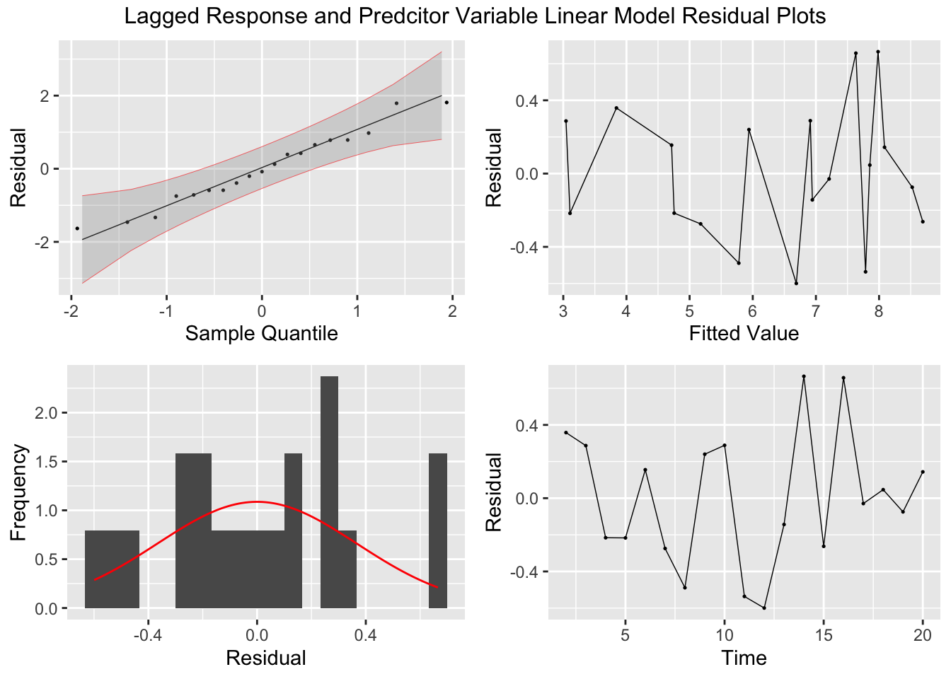
## (transformed): 1.95804 , p-value: 4.151e-01

3.4.10 Example 3.16

In this example, regressing of share on price, share(t-1), and price(t-1) eliminates any problems with autocorrelated errors.

T <- nrow(toothpaste)

(lag_toothpaste <- toothpaste[2:T,] |> mutate(lag_share = toothpaste$share[1:T-1],
                           lag_price = toothpaste$price[1:T-1]))

## # A tsibble: 19 x 5 [1]
##     time share price lag_share lag_price
##    <dbl> <dbl> <dbl>     <dbl>     <dbl>
##  1     2  4.2   0.95      3.63      0.97
##  2     3  3.33  0.99      4.2       0.95
##  3     4  4.54  0.91      3.33      0.99
##  4     5  2.89  0.98      4.54      0.91
##  5     6  4.87  0.9       2.89      0.98
##  6     7  4.9   0.89      4.87      0.9 
##  7     8  5.29  0.86      4.9       0.89
##  8     9  6.18  0.85      5.29      0.86
##  9    10  7.2   0.82      6.18      0.85
## 10    11  7.25  0.79      7.2       0.82
## 11    12  6.09  0.83      7.25      0.79
## 12    13  6.8   0.81      6.09      0.83
## 13    14  8.65  0.77      6.8       0.81
## 14    15  8.43  0.76      8.65      0.77
## 15    16  8.29  0.8       8.43      0.76
## 16    17  7.18  0.83      8.29      0.8 
## 17    18  7.9   0.79      7.18      0.83
## 18    19  8.45  0.76      7.9       0.79
## 19    20  8.23  0.78      8.45      0.76

lag_toothpaste.fit <- lag_toothpaste |>
  model(TSLM(share ~ lag_share + price + lag_price))

lag_toothpaste.fit |> report()

## Series: share 
## Model: TSLM 
## 
## Residuals:
##      Min       1Q   Median       3Q      Max 
## -0.59958 -0.23973 -0.02918  0.26351  0.66532 
## 
## Coefficients:
##             Estimate Std. Error t value Pr(>|t|)    
## (Intercept)  16.0675     6.0904   2.638   0.0186 *  
## lag_share     0.4266     0.2237   1.907   0.0759 .  
## price       -22.2532     2.4870  -8.948 2.11e-07 ***
## lag_price     7.5941     5.8697   1.294   0.2153    
## ---
## Signif. codes:  0 '***' 0.001 '**' 0.01 '*' 0.05 '.' 0.1 ' ' 1
## 
## Residual standard error: 0.402 on 15 degrees of freedom
## Multiple R-squared:  0.96,   Adjusted R-squared: 0.952
## F-statistic: 120.1 on 3 and 15 DF, p-value: 1.0367e-10

plot_residuals(augment(lag_toothpaste.fit), title = "Lagged Response and Predcitor Variable Linear Model")

## # A tibble: 1 × 3
##   .model                                      lb_stat lb_pvalue
##   <chr>                                         <dbl>     <dbl>
## 1 TSLM(share ~ lag_share + price + lag_price)  0.0612     0.805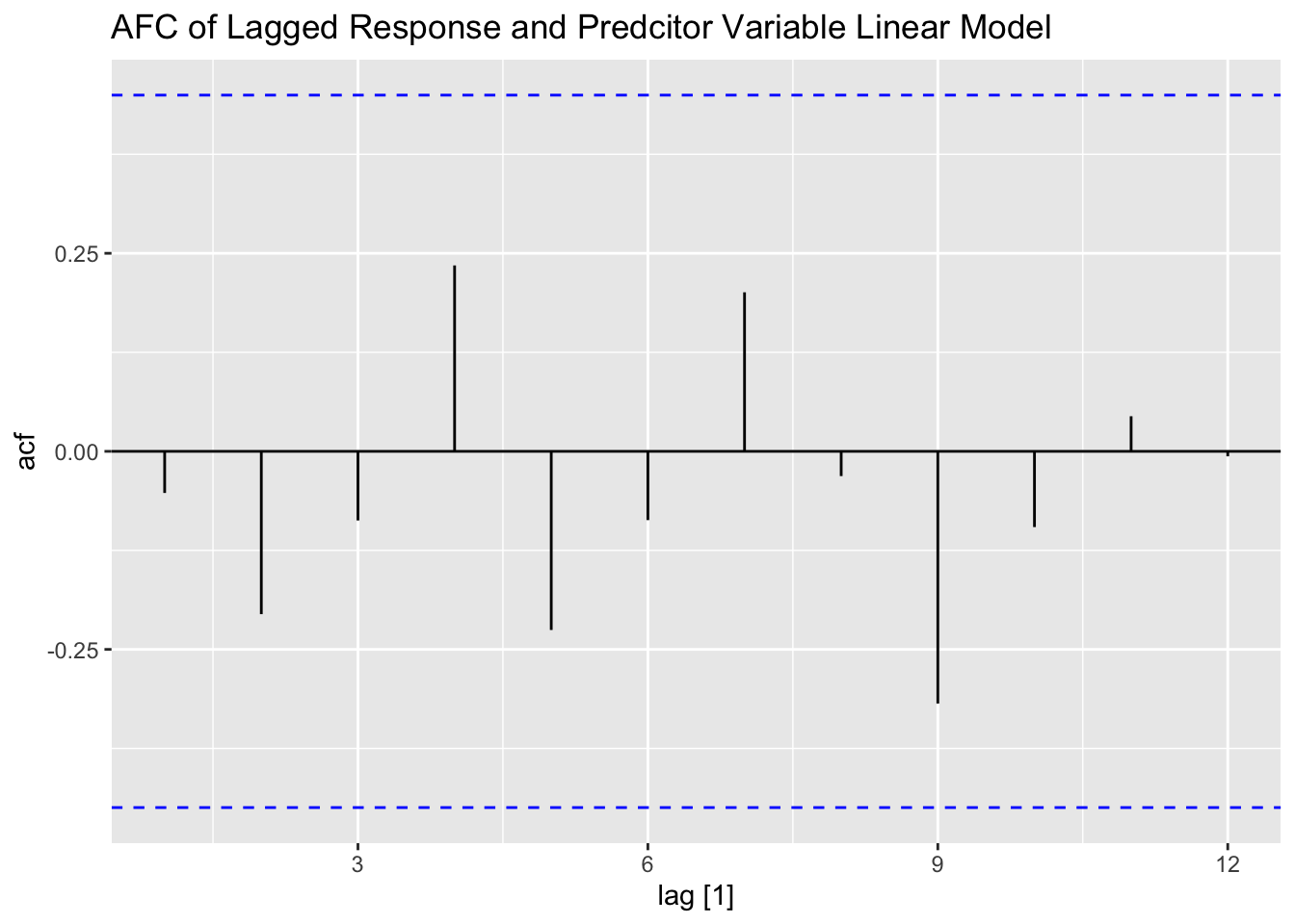

3.4.11 Maximum-Likelihood Estimation, with First-Order AR Errors

To demonstrate maximum-likelihood estimation we use functions provided through the nlme package. This package contains an ACF() function that masks the one provided through fpp3. To prevent future errors, I called all functions available through nlme using nlme:: instead of library(nlme).

tooth.fit3 <- nlme::gls(share ~ price, data = toothpaste, correlation=nlme::corARMA(p=1), method="ML")
summary(tooth.fit3)

## Generalized least squares fit by maximum likelihood
##   Model: share ~ price 
##   Data: toothpaste 
##        AIC      BIC    logLik
##   24.90475 28.88767 -8.452373
## 
## Correlation Structure: AR(1)
##  Formula: ~1 
##  Parameter estimate(s):
##       Phi 
## 0.4325871 
## 
## Coefficients:
##                 Value Std.Error   t-value p-value
## (Intercept)  26.33218  1.436305  18.33328       0
## price       -23.59030  1.673740 -14.09436       0
## 
##  Correlation: 
##       (Intr)
## price -0.995
## 
## Standardized residuals:
##         Min          Q1         Med          Q3         Max 
## -1.85194806 -0.85848738  0.08945623  0.69587678  2.03734437 
## 
## Residual standard error: 0.4074217 
## Degrees of freedom: 20 total; 18 residual

nlme::intervals(tooth.fit3)

## Approximate 95% confidence intervals
## 
##  Coefficients:
##                 lower      est.     upper
## (Intercept)  23.31462  26.33218  29.34974
## price       -27.10670 -23.59030 -20.07390
## 
##  Correlation structure:
##           lower      est.     upper
## Phi -0.04226294 0.4325871 0.7480172
## 
##  Residual standard error:
##     lower      est.     upper 
## 0.2805616 0.4074217 0.5916436

predict(tooth.fit3)

##        1        2        3        4        5        6        7        8 
## 3.449591 3.921397 2.977785 4.865009 3.213688 5.100912 5.336815 6.044524 
##        9       10       11       12       13       14       15       16 
## 6.280427 6.988136 7.695845 6.752233 7.224039 8.167651 8.403554 7.459942 
##       17       18       19       20 
## 6.752233 7.695845 8.403554 7.931748 
## attr(,"label")
## [1] "Fitted values"

# For second-order autocorrelated errors:
tooth.fit4 <- nlme::gls(share ~ price, data = toothpaste, correlation=nlme::corARMA(p=2), method="ML")
summary(tooth.fit4)

## Generalized least squares fit by maximum likelihood
##   Model: share ~ price 
##   Data: toothpaste 
##        AIC      BIC    logLik
##   26.88619 31.86485 -8.443094
## 
## Correlation Structure: ARMA(2,0)
##  Formula: ~1 
##  Parameter estimate(s):
##        Phi1        Phi2 
##  0.44554533 -0.02997286 
## 
## Coefficients:
##                 Value Std.Error   t-value p-value
## (Intercept)  26.33871  1.415367  18.60910       0
## price       -23.60022  1.649736 -14.30545       0
## 
##  Correlation: 
##       (Intr)
## price -0.995
## 
## Standardized residuals:
##         Min          Q1         Med          Q3         Max 
## -1.84716045 -0.85302820  0.09193179  0.70198216  2.04091713 
## 
## Residual standard error: 0.4073959 
## Degrees of freedom: 20 total; 18 residual

References

Montgomery, Douglas C, Cheryl L. Jennings, and Murat Kulahci. Introduction to Time Series Analysis and Forecasting. Vol. 2. Hoboken, New Jersey: John Wiley & Sons, 2016.

Montgomery, Jennings, and Kulahci, Introduction to Time Series Analysis and Forecasting.↩︎
Montgomery, Jennings, and Kulahci.↩︎

age	severity	satisfaction
55	50	68
46	24	77
30	46	96
35	48	80
59	58	43
61	60	44
74	65	26
38	42	88
27	42	75
51	50	57
53	38	56
41	30	88
37	31	88
24	34	102
42	30	88
50	48	70
58	61	52
60	71	43
62	62	46
68	38	56
70	41	59
79	66	26
63	31	52
39	42	83
49	40	75

age	severity	satisfaction
55	50	68
46	24	77
30	46	96
35	48	80
59	58	43
61	60	44
74	65	26
38	42	88
27	42	75
51	50	57
53	38	56
41	30	88
37	31	88
24	34	102
42	30	88
50	48	70
58	61	52
60	71	43
62	62	46
68	38	56
70	41	59
79	66	26
63	31	52
39	42	83
49	40	75

age	severity	satisfaction
55	50	68
46	24	77
30	46	96
35	48	80
59	58	43
61	60	44
74	65	26
38	42	88
27	42	75
51	50	57
53	38	56
41	30	88
37	31	88
24	34	102
42	30	88
50	48	70
58	61	52
60	71	43
62	62	46
68	38	56
70	41	59
79	66	26
63	31	52
39	42	83
49	40	75