6 Additional Models

This final chapter will cover additional models from the remaining chapters we have not covered in Introduction to Time Series Analysis and Forecasting as well as notable models from Forecasting: Principles and Practice past Chapter 9: ARIMA Models. Many of these models are either variants or extensions of ARIMA models covered in chapter 5 or are more recently developed models designed to handle very high frequency data (daily, sub-daily).

6.1 Chapter 6 Code

Chapter 6 contains material on intervention models and transfer function noise models. These models are in the same class as ARIMA models, but introduce other inputs that reflect changes in the process.⁴⁰

6.1.1 Example 6.5 Intervention Model for Weekly Cereal Sales Data

For the examples on intervention models we will use weekly cereal sales data from CerealSales.csv. First, I read in cereal sales data, rename the variables, and declare it as a tsibble. The time variable does not need to be modified to be used as an index, as time is kept periodically. In this data, at week 88 a rival company introduces a similar product into the market.

(cereal <- read_csv("data/CerealSales.csv") |> 
  rename(time = 1, sales = 2) |> 
  as_tsibble(index = time))

## Rows: 104 Columns: 2
## ── Column specification ───────────────────────────────────────
## Delimiter: ","
## dbl (2): Week, Sales
## 
## ℹ Use `spec()` to retrieve the full column specification for this data.
## ℹ Specify the column types or set `show_col_types = FALSE` to quiet this message.

## # A tsibble: 104 x 2 [1]
##     time  sales
##    <dbl>  <dbl>
##  1     1 102450
##  2     2  98930
##  3     3  91550
##  4     4 111940
##  5     5 103380
##  6     6 112120
##  7     7 105780
##  8     8 103000
##  9     9 111920
## 10    10 106170
## # ℹ 94 more rows

I then plot the data and mark week 88, when the rival product hits the market. The data before week 88 has a clear upward trend. This changes after week 88. Often, data can have a point where a significant event not captured within the data changes the trend and/or seasonality of the data. A good example of this is housing sales data from 2000 to 2019. In this middle of this data the housing market crash and resulting economic effects can be reasonably expected to have a large impact on the data after this event.

cereal |>
  ggplot(aes(x = time, y = sales)) +
  geom_point(size = 0.5) +
  geom_line() +
  geom_vline(aes(xintercept = 88)) + 
  labs(title = "Plot of Cereal Sales over Time")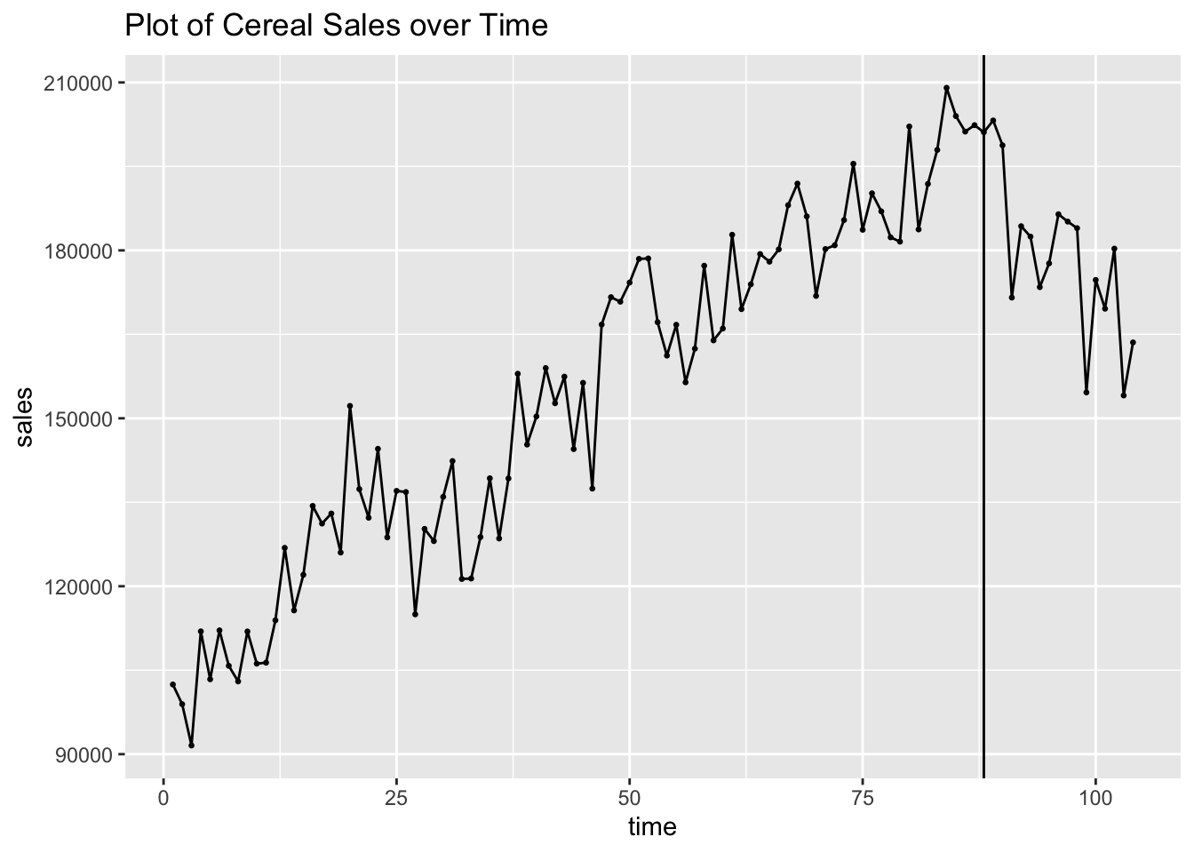

To identify the ARMA for pre-intervention data, I plot the ACF and PACF of the data. The ACF and PACF show that there is clearly lingering autocorrelation and that the data could possibly benefit from differencing.

cereal |>
  filter(time <= 87) |>
  ACF(sales, lag_max = 25) |>
  autoplot() +
  labs(title = "ACF of the Pre-Intervention Cereal Sales Data")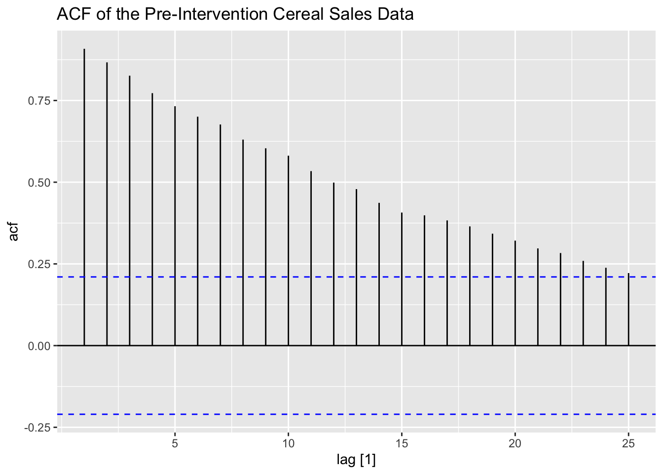

cereal |>
  filter(time <= 87) |>
  PACF(sales, lag_max = 25) |>
  autoplot() + 
  labs(title = "PACF of the Pre-Intervention Cereal Sales Data")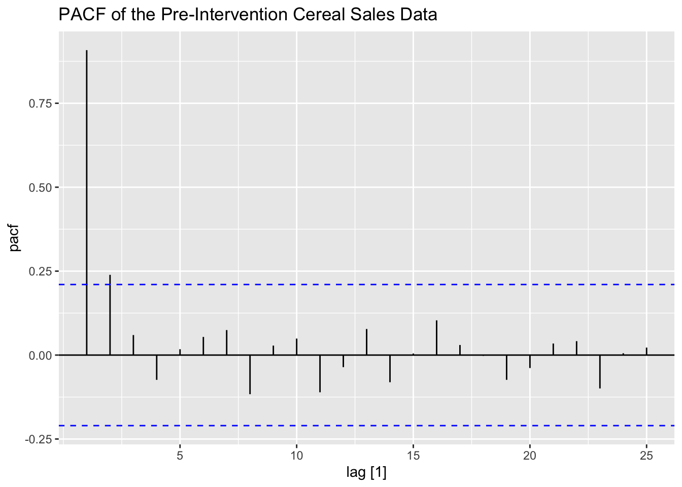

I then take the first difference of the data and examine the pre-intervention first differenced ACF and PACF of the data. I also create an indicator variable, which equals zero before week 88 and equals one after. This will serve as a dummy variable indicating if the competitor has entered the market yet.

#create the difference variable and intervention variable
(cereal <- cereal |>
  mutate(diff = difference(sales, 1),
         ind = case_when(time <= 87 ~ 0, 
                         time > 87 ~ 1)))

## # A tsibble: 104 x 4 [1]
##     time  sales  diff   ind
##    <dbl>  <dbl> <dbl> <dbl>
##  1     1 102450    NA     0
##  2     2  98930 -3520     0
##  3     3  91550 -7380     0
##  4     4 111940 20390     0
##  5     5 103380 -8560     0
##  6     6 112120  8740     0
##  7     7 105780 -6340     0
##  8     8 103000 -2780     0
##  9     9 111920  8920     0
## 10    10 106170 -5750     0
## # ℹ 94 more rows

cereal |>
  filter(time <= 87) |>
  ACF(diff, lag_max = 25) |>
  autoplot() + 
  labs(title = "ACF of First Differenced Cereal Sales Data before Intervention")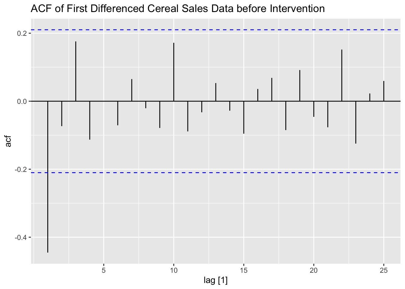

cereal |>
  filter(time <= 87) |>
  PACF(diff, lag_max = 25) |>
  autoplot() + 
  labs(title = "PACF of First Differenced Cereal Sales Data before Intervention")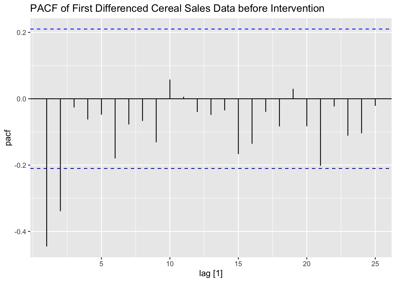

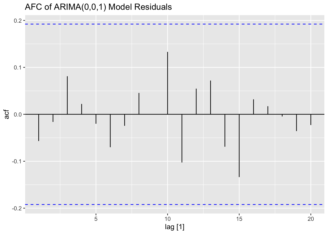
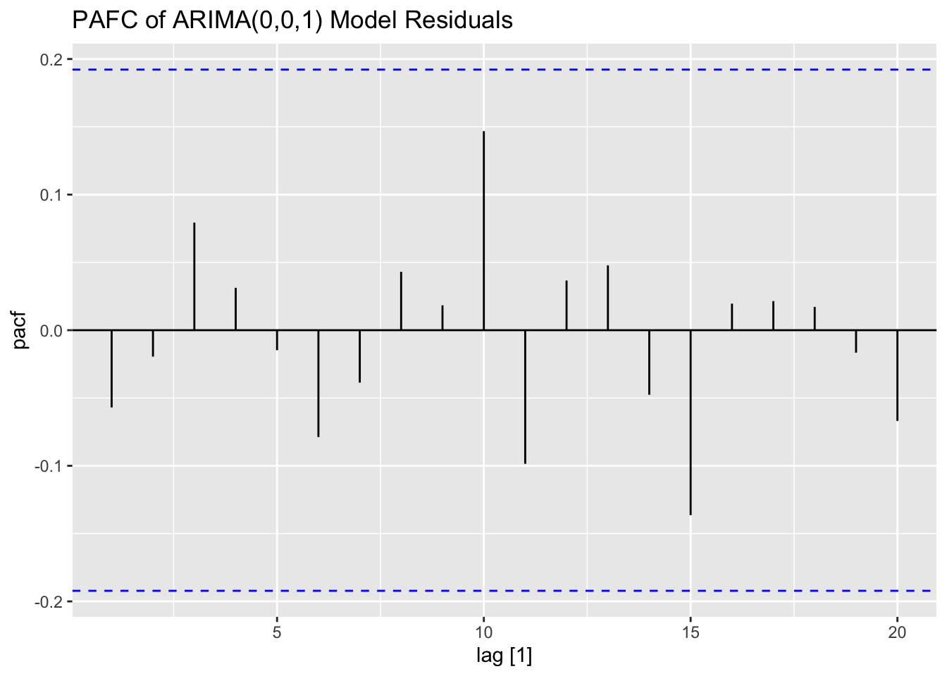
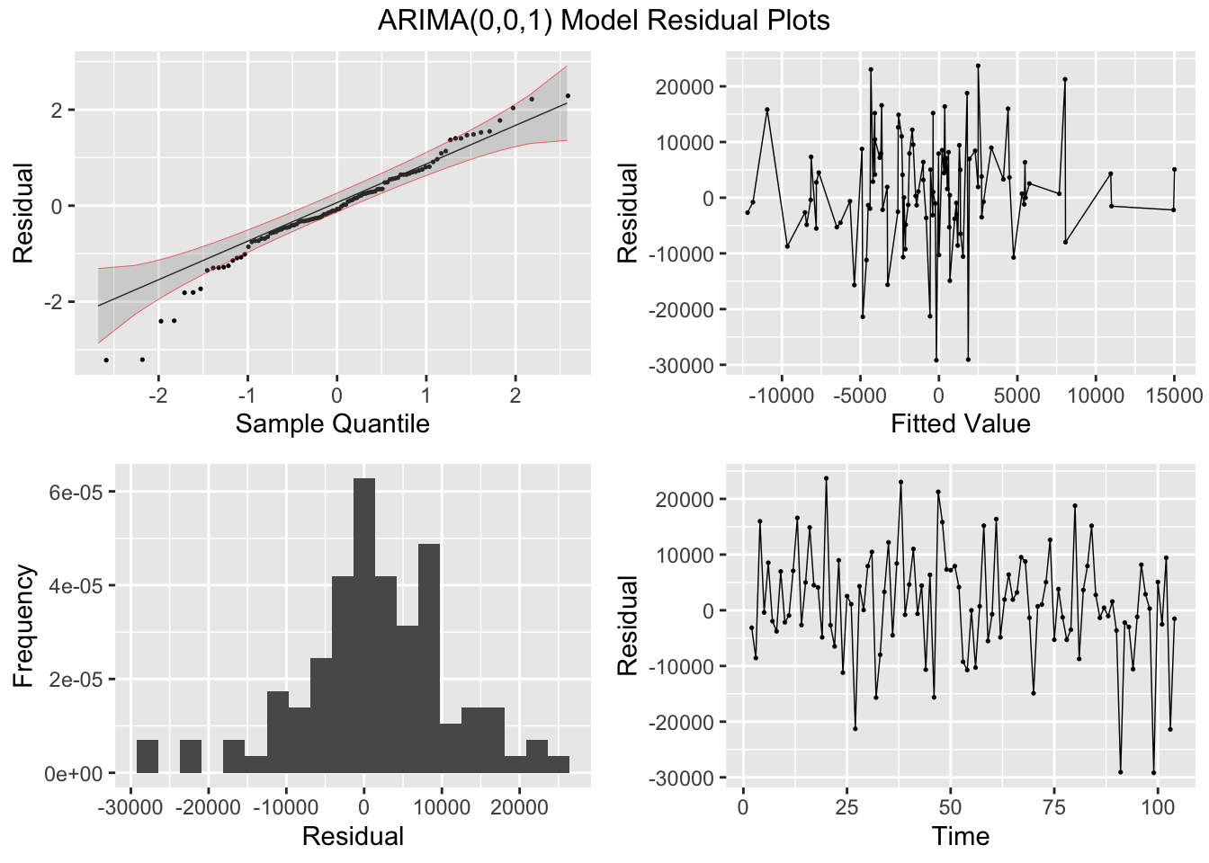
After examining the ACF and PACF, I create an linear model regressing the differenced data on the indicator variable with ARIMA(0,0,1) errors. For comparison, I allow the algorithm to select the best ARIMA model for the differenced data according to AICc. The linear model with ARIMA errors performs slightly better than the ARIMA model selected by the algorithm.

cereal.fit <- cereal |>
  model(int = ARIMA(diff ~ 0 + pdq(0,0,1) + ind),
        best = ARIMA(diff, stepwise = FALSE))

cereal.fit |> select(best) |> report()

## Series: diff 
## Model: ARIMA(0,0,1) 
## 
## Coefficients:
##           ma1
##       -0.5144
## s.e.   0.0772
## 
## sigma^2 estimated as 96667735:  log likelihood=-1093.22
## AIC=2190.45   AICc=2190.57   BIC=2195.74

cereal.fit |> select(int) |> report()

## Series: diff 
## Model: LM w/ ARIMA(0,0,1) errors 
## 
## Coefficients:
##           ma1        ind
##       -0.5571  -2369.901
## s.e.   0.0757   1104.530
## 
## sigma^2 estimated as 93672303:  log likelihood=-1091.13
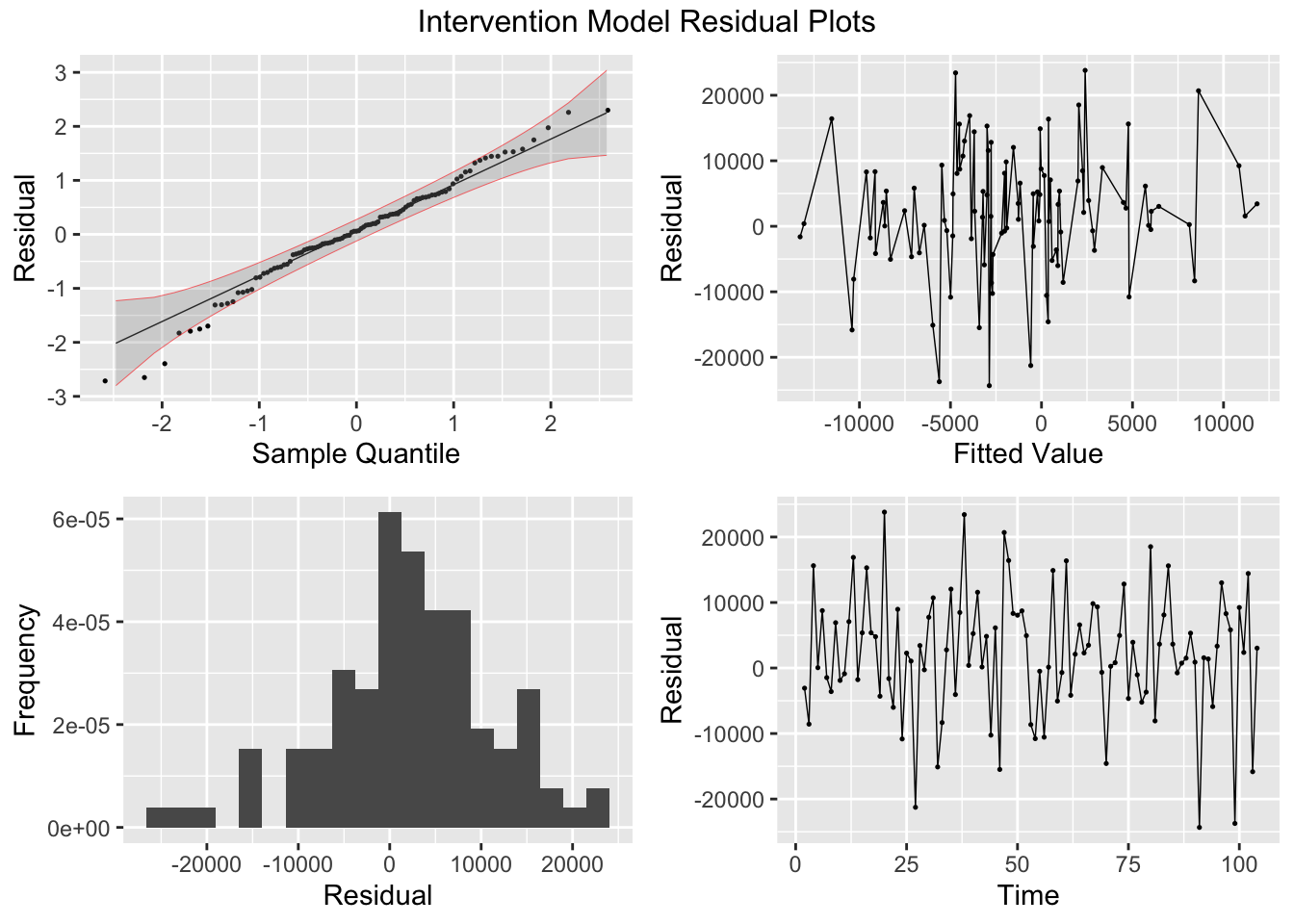
## AIC=2188.27   AICc=2188.51   BIC=2196.2

I then plot and examine the residuals of the model using plot_residuals() and plot both of the models with the original data. I look at the measures of accuracy using the accuracy function as well. The residuals from both models do not have any lingering autocorrelation. The intervention model appears to perform slightly better than the straight ARIMA model.

plot_residuals(augment(cereal.fit), title = c("Intervention Model", "ARIMA(0,0,1) Model"))

## # A tibble: 2 × 3
##   .model lb_stat lb_pvalue
##   <chr>    <dbl>     <dbl>
## 1 best     0.344     0.558
## 2 int      0.935     0.333
## # A tibble: 2 × 3
##   .model kpss_stat kpss_pvalue
##   <chr>      <dbl>       <dbl>
## 1 best      0.360       0.0942
## 2 int       0.0841      0.1

## NULL

augment(cereal.fit) |> autoplot(.fitted) + autolayer(cereal, diff)

## Warning: Removed 2 rows containing missing values (`geom_line()`).

## Warning: Removed 1 row containing missing values (`geom_line()`).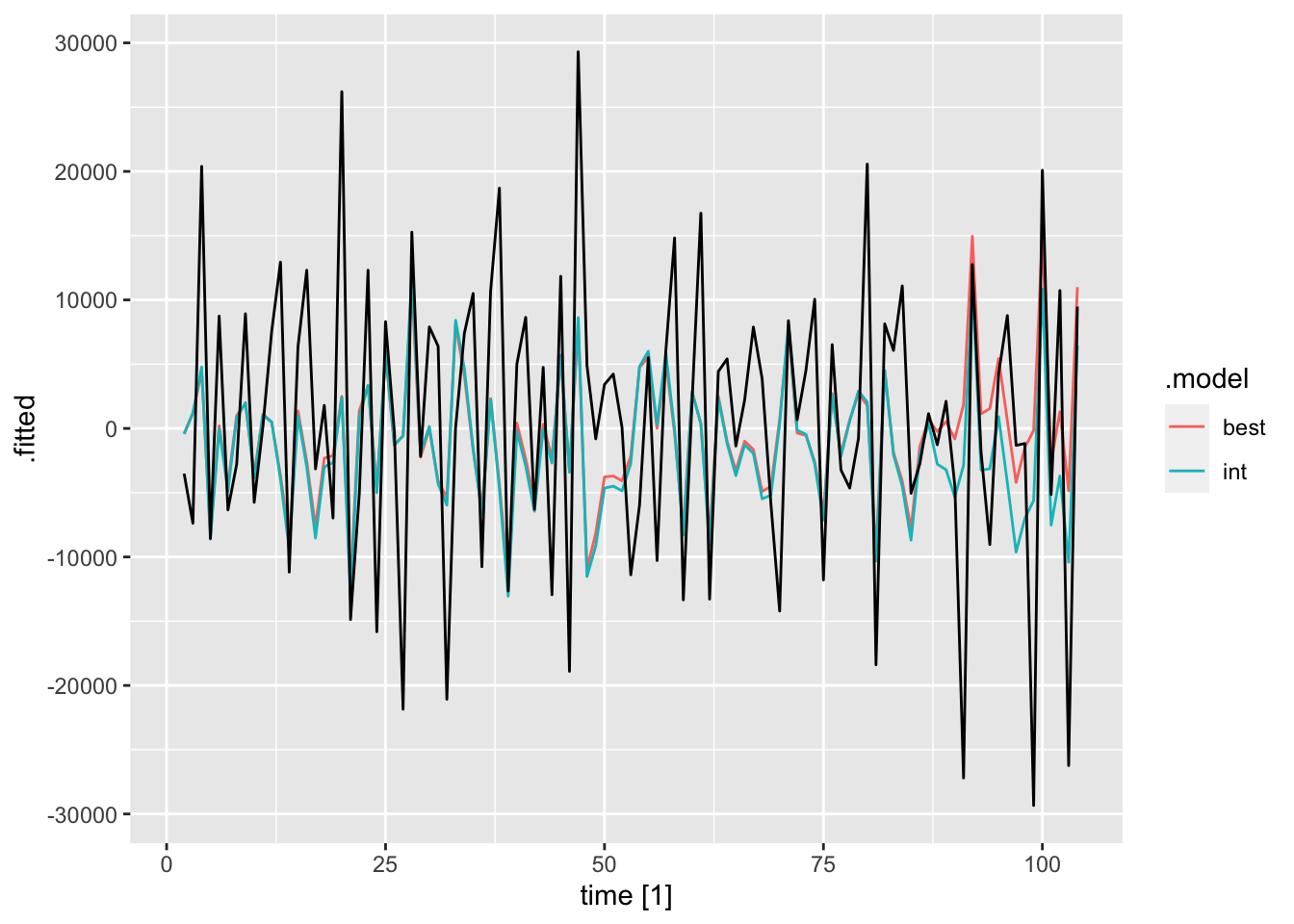

dig <- function(x){round(x, digits = 3)} # function for mutate if to round digits to 3 decimals
accuracy(cereal.fit) |> mutate_if(is.numeric, dig) |> gt()

.model	.type	ME	RMSE	MAE	MPE	MAPE	MASE	RMSSE	ACF1
int	Training	2204.559	9631.348	7399.349	0.301	277.564	0.484	0.504	-0.094
best	Training	1252.384	9831.975	7355.590	7.420	252.298	0.481	0.515	-0.057

6.1.2 Example 6.2: Transfer Function Noise Model for Chemical Process Viscosity

For this example, I will be using the chemical process viscocity data from ChemicalViscocity.csv. I use row_number() to create a periodic time variable and then assign that variable as the index when making it into a tsibble.

(visc <- read_csv("data/ChemicalViscosity.csv") |>
   rename(temp = 1, visc = 2) |> 
   mutate(time = row_number()) |> 
   as_tsibble(index = time))

## Rows: 100 Columns: 2
## ── Column specification ───────────────────────────────────────
## Delimiter: ","
## dbl (2): temperature, viscosity
## 
## ℹ Use `spec()` to retrieve the full column specification for this data.
## ℹ Specify the column types or set `show_col_types = FALSE` to quiet this message.

## # A tsibble: 100 x 3 [1]
##     temp  visc  time
##    <dbl> <dbl> <int>
##  1  0.17  0.3      1
##  2  0.13  0.18     2
##  3  0.19  0.09     3
##  4  0.09  0.06     4
##  5  0.03  0.3      5
##  6  0.11  0.44     6
##  7  0.15  0.46     7
##  8 -0.02  0.44     8
##  9  0.07  0.34     9
## 10  0     0.23    10
## # ℹ 90 more rows

I then plot both the temperature and viscosity variables over time for visual analysis.

visc |>
  ggplot(aes(x = time, y = temp)) +
  geom_point(size = 0.5) +
  geom_line() + 
  labs(title = "Plot of Temperature over Time",
       y = "temperature")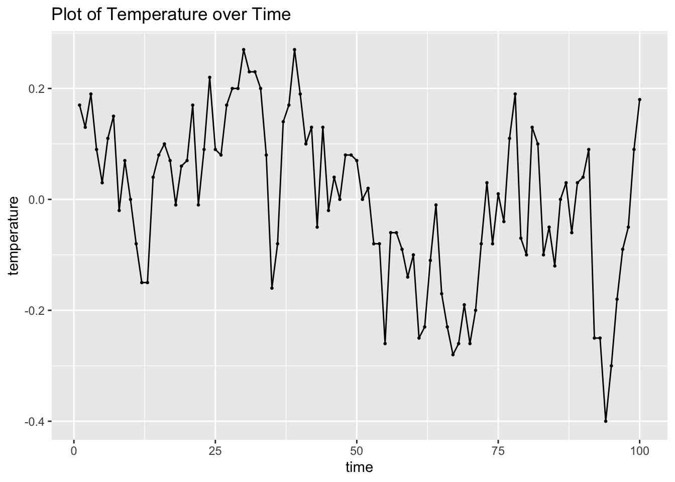

visc |>
  ggplot(aes(x = time, y = visc)) +
  geom_point(size = 0.5) +
  geom_line() + 
  labs(title = "Plot of Chemical Viscocity over Time",
       y = "viscocity")

Next is prewhitening. To identify a model for temperature, I plot its ACF and PACF below.

visc |>
  ACF(temp, lag_max = 25) |>
  autoplot() +
  labs(title = "ACF Plot of Temperature Data")

visc |>
  PACF(temp, lag_max = 25) |>
  autoplot() +
  labs(title = "PACF Plot of Temperature Data")

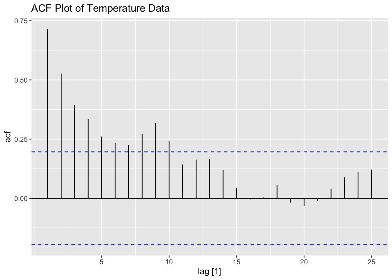
I then fit an AR(1) model to temperature. Recall, to make sure a model is exactly as specified, you must include all components (constant, pdq, and PDQ). The coefficient in the AR(1) model is statistically significant.

visc.temp.fit <- visc |>
  model(ar1 = ARIMA(temp ~ 0 + pdq(1,0,0) + PDQ(0,0,0)))

visc.temp.fit |> tidy() |> mutate_if(is.numeric, dig) |> gt()

.model	term	estimate	std.error	statistic	p.value
ar1	ar1	0.729	0.069	10.633	0

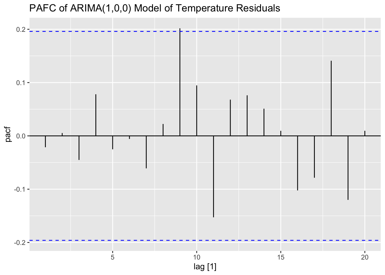
I then examine the ACF, PACF, and residuals of the AR(1) model of temperature. The residuals do not have any lingering autocorrelation.

augment(visc.temp.fit) |> plot_residuals(title = "ARIMA(1,0,0) Model of Temperature")

## # A tibble: 1 × 3
##   .model lb_stat lb_pvalue
##   <chr>    <dbl>     <dbl>
## 1 ar1     0.0468     0.829
## # A tibble: 1 × 3
##   .model kpss_stat kpss_pvalue
##   <chr>      <dbl>       <dbl>
## 1 ar1        0.335         0.1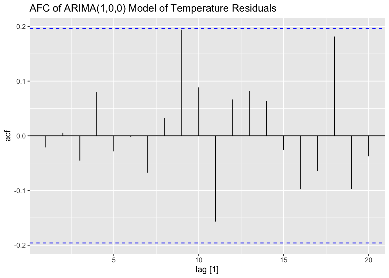

## NULL

Next, I prewhiten both series using an AR(1) coefficient of 0.73 from the model of temperature above. I calculate \(\alpha_{t}\) and \(\beta_{t}\) within mutate() and use lag() to multiply the previous observation by the coefficient. Finally, I plot the CCF of \(\alpha_{t}\) and \(\beta_{t}\).

(visc <- visc |>
  mutate(alpha = temp - 0.73*lag(temp, n = 1),
         beta = visc - 0.73*lag(visc, n = 1)))

## # A tsibble: 100 x 5 [1]
##     temp  visc  time   alpha     beta
##    <dbl> <dbl> <int>   <dbl>    <dbl>
##  1  0.17  0.3      1 NA      NA      
##  2  0.13  0.18     2  0.0059 -0.039  
##  3  0.19  0.09     3  0.0951 -0.0414 
##  4  0.09  0.06     4 -0.0487 -0.00570
##  5  0.03  0.3      5 -0.0357  0.256  
##  6  0.11  0.44     6  0.0881  0.221  
##  7  0.15  0.46     7  0.0697  0.139  
##  8 -0.02  0.44     8 -0.130   0.104  
##  9  0.07  0.34     9  0.0846  0.0188 
## 10  0     0.23    10 -0.0511 -0.0182 
## # ℹ 90 more rows

ralbe <- visc |>
  CCF(alpha, beta) 

ralbe |>
  autoplot() + 
  geom_vline(aes(xintercept = 0), color = "blue") +
  labs(title = "CCF of alpha(t) and beta(t)")

To obtain estimates of \(\hat v_{t}\), I use mutate() to create a vhat variable in the CCF data frame saved as ralbe. I then plot \(\hat v_{t}\) in a similar style as an ACF, PACF, or CCF. The blue line indicates the competitor entering the market. It looks very similar in shape to the CCF above because \(\hat v_{t}\) is a function of the CCF.

library(latex2exp)
(ralbe <- ralbe |> 
  mutate(vhat = sqrt(var(visc$beta[2:100])/var(visc$alpha[2:100]))*ccf))

## # A tsibble: 33 x 3 [1]
##         lag     ccf    vhat
##    <cf_lag>   <dbl>   <dbl>
##  1      -16 -0.0521 -0.0972
##  2      -15  0.121   0.225 
##  3      -14 -0.0461 -0.0861
##  4      -13 -0.0407 -0.0760
##  5      -12 -0.107  -0.199 
##  6      -11 -0.0564 -0.105 
##  7      -10 -0.0105 -0.0196
##  8       -9  0.0543  0.101 
##  9       -8 -0.0219 -0.0408
## 10       -7  0.117   0.218 
## # ℹ 23 more rows

ralbe |> 
  ggplot(aes(x = lag, y = vhat)) + 
  geom_hline(aes(yintercept = 0)) +
  geom_vline(aes(xintercept = 0), color = "blue") +
  geom_segment(aes(xend = lag, yend = 0)) + 
  labs(title = "Impulse Control", y = "v_hat")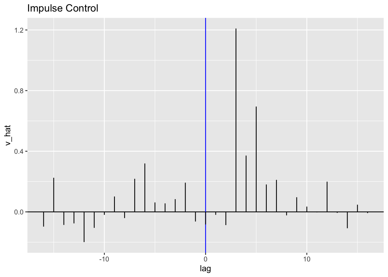

I then model the noise using the estimates given in the example. To do this, I create a vector of zeros, and then loop from the 4th element to the end, calculating Nhat. After calculations, I change the first three element from 0 to NA and then append the vector to the visc data frame.

T <-length(visc$temp)
Nhat <- vector(mode = "numeric", length = T)
for (i in 4:T){
    Nhat[i] <- visc$visc[i] + 0.31*(Nhat[i-1]-visc$visc[i-1]) + 0.48*(Nhat[i-2]-visc$visc[i-2]) + 1.21*visc$temp[i-3]
}
Nhat[1:3] <- NA # 1:3 must be 0 in for loop for calculations
#must make those NA so then can mutate into visc
(visc <- visc |>
  mutate(Nhat = Nhat))

## # A tsibble: 100 x 6 [1]
##     temp  visc  time   alpha     beta   Nhat
##    <dbl> <dbl> <int>   <dbl>    <dbl>  <dbl>
##  1  0.17  0.3      1 NA      NA       NA    
##  2  0.13  0.18     2  0.0059 -0.039   NA    
##  3  0.19  0.09     3  0.0951 -0.0414  NA    
##  4  0.09  0.06     4 -0.0487 -0.00570  0.151
##  5  0.03  0.3      5 -0.0357  0.256    0.442
##  6  0.11  0.44     6  0.0881  0.221    0.758
##  7  0.15  0.46     7  0.0697  0.139    0.736
##  8 -0.02  0.44     8 -0.130   0.104    0.714
##  9  0.07  0.34     9  0.0846  0.0188   0.691
## 10  0     0.23    10 -0.0511 -0.0182   0.652
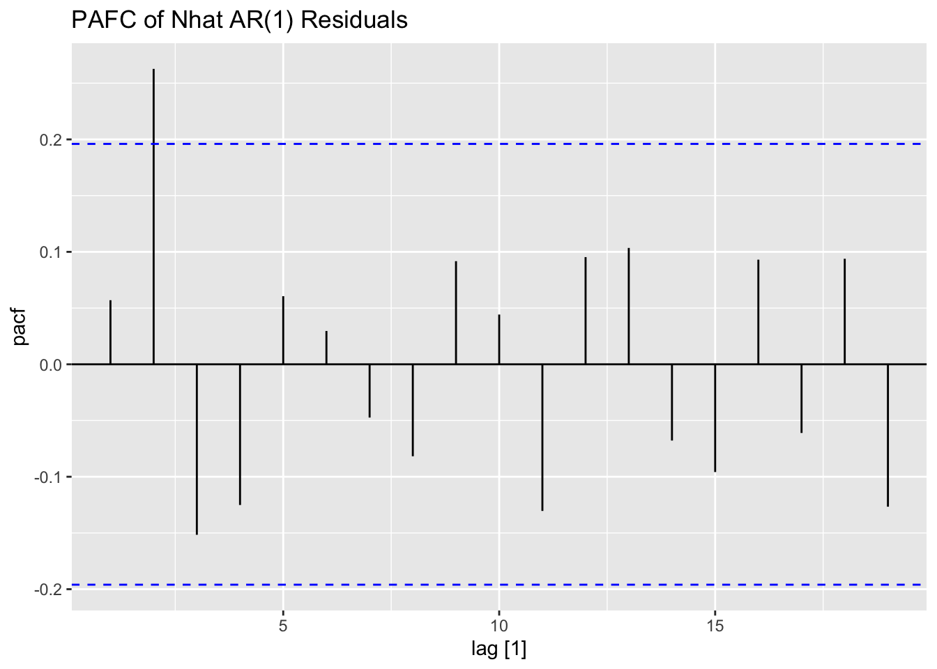
## # ℹ 90 more rows

I look at the ACF and PACF of the newly calculated Nhat to determine possible models.

visc |> ACF(Nhat) |> autoplot()

visc |> PACF(Nhat) |> autoplot()

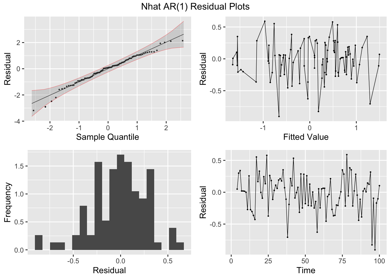
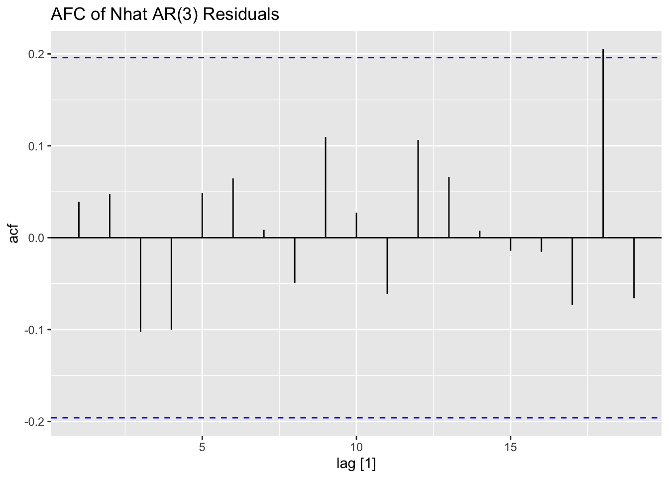
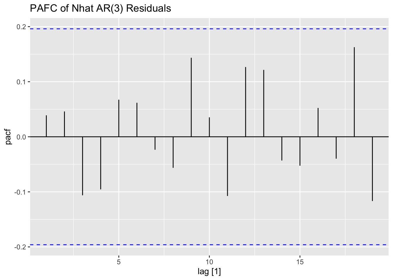
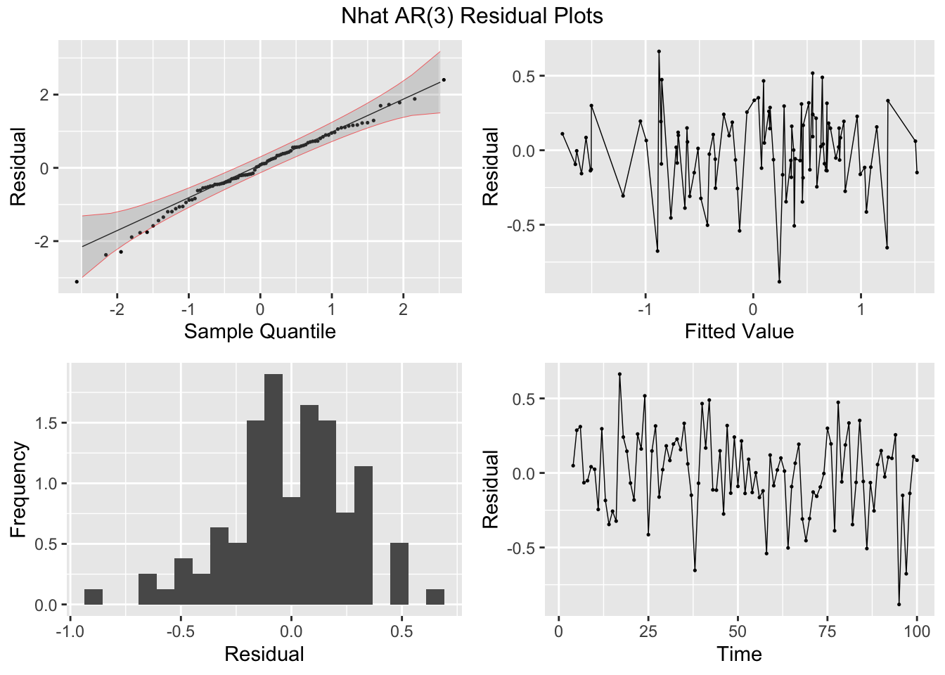
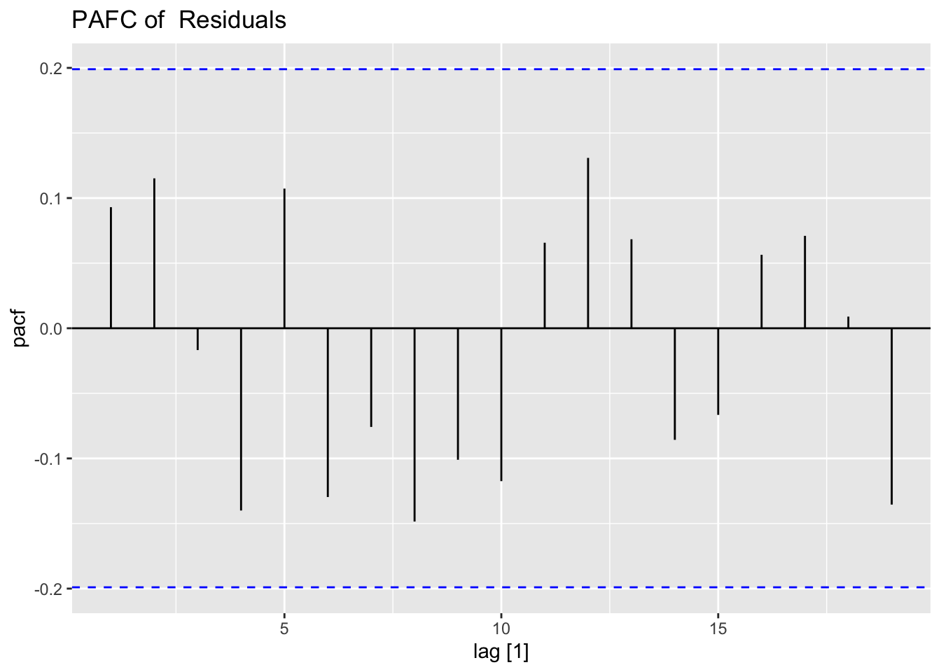
Next, I fit AR(1) and AR(3) models (without constants) to Nhat and plot the residuals of both models for analysis. The AR(1) model has lingering autocorrelation but the coefficients of the AR(3) model are not siginificant, so the AR(1) model is deemed to be the appropriate model.⁴¹

nhat.models <- visc |>
  model(ar1 = ARIMA(Nhat ~ 0 + pdq(1,0,0) + PDQ(0,0,0)),
        ar3 = ARIMA(Nhat ~ 0 + pdq(3,0,0) + PDQ(0,0,0)))

nhat.models |> select(ar1) |> report()

## Series: Nhat 
## Model: ARIMA(1,0,0) 
## 
## Coefficients:
##          ar1
##       0.9452
## s.e.  0.0319
## 
## sigma^2 estimated as 0.08013:  log likelihood=-17.33
## AIC=38.66   AICc=38.78   BIC=43.87

nhat.models |> select(ar3) |> report()

## Series: Nhat 
## Model: ARIMA(3,0,0) 
## 
## Coefficients:
##          ar1     ar2      ar3
##       0.9838  0.2249  -0.2893
## s.e.  0.0964  0.1369   0.0989
## 
## sigma^2 estimated as 0.07483:  log likelihood=-13.12
## AIC=34.24   AICc=34.66   BIC=44.66

augment(nhat.models) |> plot_residuals(title = c("Nhat AR(1)", "Nhat AR(3)"))

## # A tibble: 2 × 3
##   .model lb_stat lb_pvalue
##   <chr>    <dbl>     <dbl>
## 1 ar1      0.325     0.569
## 2 ar3      0.152     0.697
## # A tibble: 2 × 3
##   .model kpss_stat kpss_pvalue
##   <chr>      <dbl>       <dbl>
## 1 ar1        0.287      0.1   
## 2 ar3        0.410      0.0727

## NULL

The transfer function noise model is not included in fable, so I will be using functions from the TSA package to create this model. The tentative overall model is shown in the equation below:

\[ y_{t} = \frac{w_{0}}{1 - \delta_{1}B - \delta_{2}B^{2}}x_{t-3} + \frac{1}{1 - \phi_{1}B} \epsilon_{t} \]⁴²

Below, I define the components of the model and bind them together in a data frame before using arimax() to create the model.

ts.xt  <- ts(visc$temp)
lag3.x <- stats::lag(ts.xt, -3)
ts.yt  <- ts(visc$visc)
dat3   <- cbind(ts.xt,lag3.x,ts.yt)
dimnames(dat3)[[2]] <- c("xt","lag3x","yt")
data2 <- na.omit(as.data.frame(dat3))
#Input arguments
#order: determines the model for the error component, 
# i.e. the order of the ARIMA model for y(t) if there were no x(t)
#xtransf: x(t)
#transfer: the orders (r and s) of the transfer function
visc.tf<-TSA::arimax(data2$yt, 
                     order=c(1,0,0), 
                     xtransf=data.frame(data2$lag3x), 
                     transfer=list(c(2,0)), 
                     include.mean = FALSE)
visc.tf

## 
## Call:
## TSA::arimax(x = data2$yt, order = c(1, 0, 0), include.mean = FALSE, xtransf = data.frame(data2$lag3x), 
##     transfer = list(c(2, 0)))
## 
## Coefficients:
##          ar1  data2.lag3x-AR1  data2.lag3x-AR2  data2.lag3x-MA0
##       0.8295           0.3414           0.2667           1.3276
## s.e.  0.0642           0.0979           0.0934           0.1104
## 
## sigma^2 estimated as 0.0123:  log likelihood = 75.09,  aic = -142.18

To analyze the residuals of a model outside of fable using plot_residuals(), the residuals must be organized similarly to the results of augment(). After creating a tsibble containing the necessary information, I run the function. I also create a CCF of the residuals and alpha as well.

(resid <- tsibble(
  .model = "TR-N",
  time = visc$time[4:100],
  .fitted = fitted(visc.tf),
  .resid = residuals(visc.tf),
  index = time
))

## # A tsibble: 97 x 4 [1]
##    .model  time .fitted    .resid
##    <chr>  <int>   <dbl>     <dbl>
##  1 TR-N       4  0.153  -0.0925  
##  2 TR-N       5  0.112   0.188   
##  3 TR-N       6  0.439   0.000552
##  4 TR-N       7  0.357   0.103   
##  5 TR-N       8  0.370   0.0696  
##  6 TR-N       9  0.472  -0.132   
##  7 TR-N      10  0.394  -0.164   
##  8 TR-N      11  0.0657  0.00431 
##  9 TR-N      12  0.160   0.0499  
## 10 TR-N      13  0.0986 -0.0686  
## # ℹ 87 more rows

plot_residuals(resid)

## # A tibble: 1 × 2
##   lb_stat lb_pvalue
##     <dbl>     <dbl>
## 1   0.865     0.352
## # A tibble: 1 × 2
##   kpss_stat kpss_pvalue
##       <dbl>       <dbl>
## 1    0.0632         0.1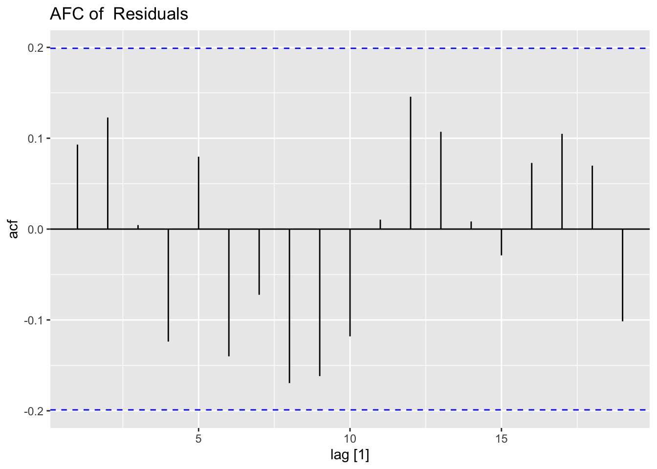

## NULL

resid |>
  left_join(visc, by = join_by(time)) |>
  CCF(alpha, .resid) |>
  autoplot() +
  labs(title = "CCF of alpha(t) and Residuals of TF-N Model")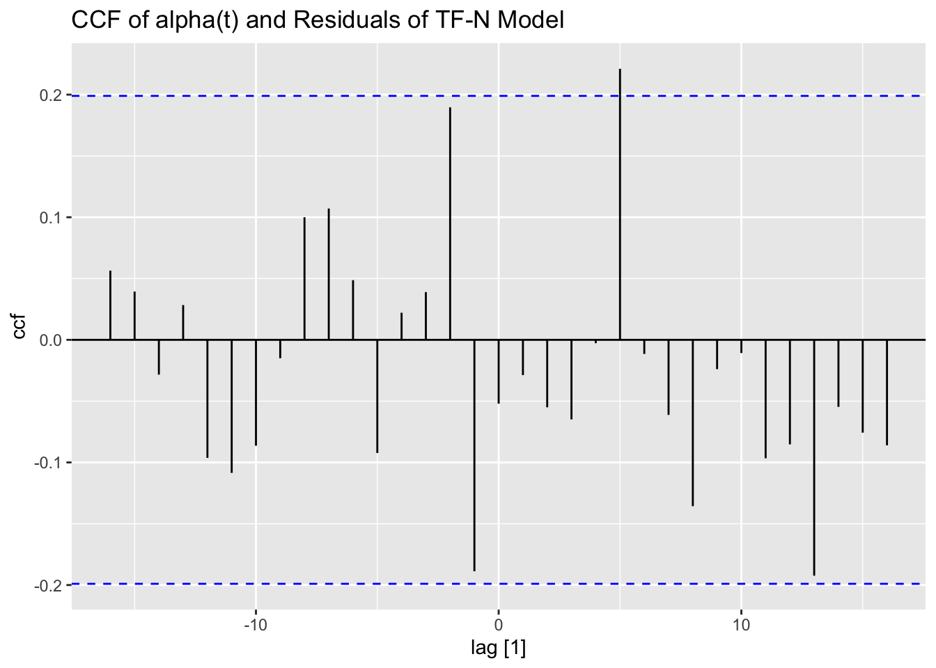

6.2 GARCH Models

Generalized Autoregressive Conditional Heteroskedastic models relax the assumption of a constant variance for the residuals. In the code chunk below, I demonstrate a simulated GARCH Model. The garch() function, used to create these models, is part of the tseries package as GARCH models are not included in fable.

library(tseries)

## Registered S3 method overwritten by 'quantmod':
##   method            from
##   as.zoo.data.frame zoo

set.seed(1)
alpha0 <- 0.1
alpha1 <- 0.4
beta1 <- 0.2
w <- rnorm(10000)
a <- rep(0, 10000)
h <- rep(0, 10000)
for (i in 2:10000) {
  h[i] <- alpha0 + alpha1 * (a[i - 1]^2) + beta1 * h[i - 1] # this is the data generating process
  a[i] <- w[i] * sqrt(h[i])
}

ACF(ts(a) |> as_tsibble()) |>
  autoplot() +
  labs(title = "ACF of Simulated Series")

## Response variable not specified, automatically selected `var = value`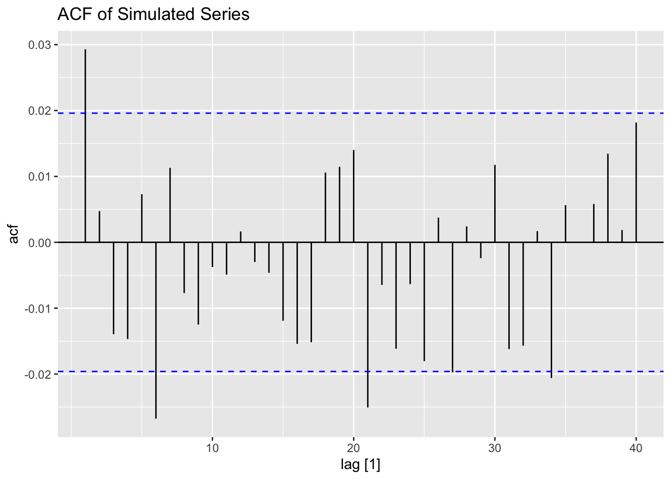

ACF(ts(a^2) |> as_tsibble()) |> 
  autoplot() +
  labs(title = "ACF of Simulated Series Squared")

## Response variable not specified, automatically selected `var = value`

(a.garch <- garch(a, grad = "numerical", trace = FALSE))

## 
## Call:
## garch(x = a, grad = "numerical", trace = FALSE)
## 
## Coefficient(s):
##      a0       a1       b1  
## 0.09876  0.36659  0.24415

# code for the GARCH model
confint(a.garch)

##        2.5 %    97.5 %
## a0 0.0882393 0.1092903
## a1 0.3307897 0.4023932
## b1 0.1928344 0.2954660

6.2.1 S&P500 Example

In this example we will be using the daily S&P 500 index data from 1990 to 1999 included in the MASS package. Note the data only includes trading days not all days. I read in the datato a tibble, create a periodic time variable, and make that variable the index of a tsibble containing the data. I also create a version of the data as a time series, as the functions for garch models are not part of fable and require a time series object instead of a tsibble.

#library(MASS)
(sp <- tibble(sp500 = MASS::SP500) |>
  mutate(time = row_number()) |>
  as_tsibble(index = time))

## # A tsibble: 2,780 x 2 [1]
##     sp500  time
##     <dbl> <int>
##  1 -0.259     1
##  2 -0.865     2
##  3 -0.980     3
##  4  0.450     4
##  5 -1.19      5
##  6 -0.663     6
##  7  0.351     7
##  8 -2.50      8
##  9 -0.866     9
## 10  1.11     10
## # ℹ 2,770 more rows

sp500 <- ts(MASS::SP500)

Next, I plot the S&P 500 data. The data has 2,780 observations, so the plot is very overcrowded with points.

sp |>
  ggplot(aes(x = time, y = sp500)) +
  geom_point(size = 0.5) +
  geom_line() + 
  labs(title = "Plot of S&P 500 over Time",
       y = "index")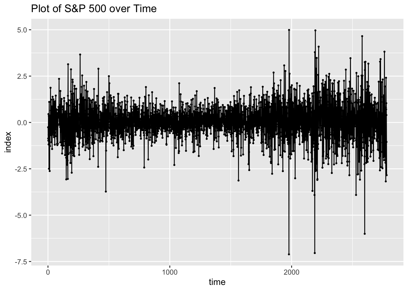

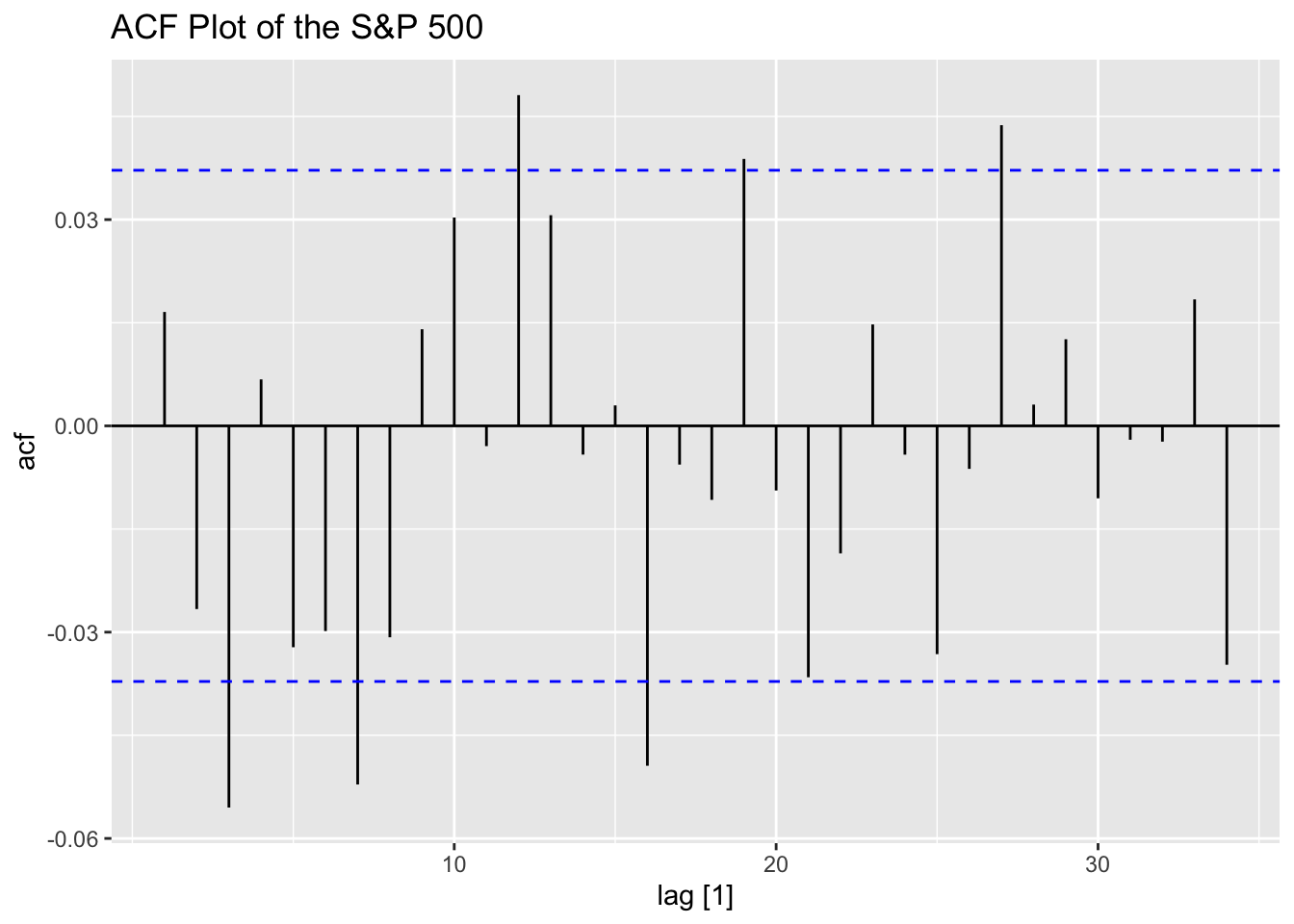
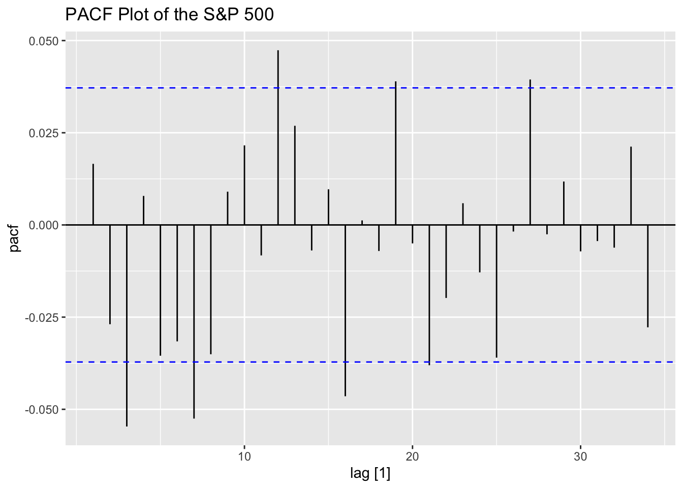
Looking at the ACF and PACF of the data, the data clearly has lingering autocorrelation.

sp |> 
  ACF(sp500) |>
  autoplot() + 
  labs(title = "ACF Plot of the S&P 500")

sp |> 
  PACF(sp500) |>
  autoplot() + 
  labs(title = "PACF Plot of the S&P 500")

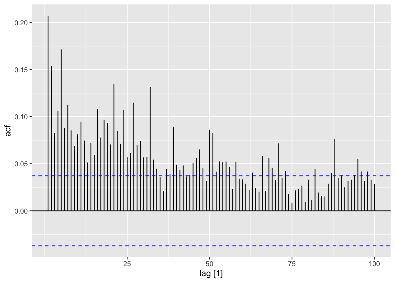
Next, I take the ACF of the squared residuals of the mean.

sp |>
  ACF((sp500 - mean(sp500))^2, lag_max = 100) |>
  autoplot()

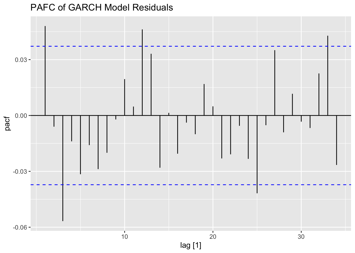
To fit a GARCH model to the data I use the garch() function. I then take the residuals and fitted values and make a tsibble that can be used with plot_residuals() to analyze the residuals. I additionally create an ACF plot of the square of the residuals.

sp.garch <- garch(sp500, trace = F)
sp.garch

## 
## Call:
## garch(x = sp500, trace = F)
## 
## Coefficient(s):
##       a0        a1        b1  
## 0.004292  0.050054  0.946773

(sp.garch.resid <- tibble(.model = "garch",
                          .resid = as.vector(sp.garch[["residuals"]]),
                          .fitted = as.vector(sp.garch[["fitted.values"]][,1])) |>
  mutate(time = row_number()) |>
  filter(time != 1) |>
  as_tsibble(index = time))

## # A tsibble: 2,779 x 4 [1]
##    .model .resid .fitted  time
##    <chr>   <dbl>   <dbl> <int>
##  1 garch  -0.762    1.14     2
##  2 garch  -0.873    1.12     3
##  3 garch   0.403    1.12     4
##  4 garch  -1.08     1.09     5
##  5 garch  -0.604    1.10     6
##  6 garch   0.324    1.08     7
##  7 garch  -2.36     1.06     8
##  8 garch  -0.739    1.17     9
##  9 garch   0.955    1.16    10
## 10 garch  -0.855    1.16    11
## # ℹ 2,769 more rows

plot_residuals(sp.garch.resid, title = "GARCH Model")

## # A tibble: 1 × 2
##   lb_stat lb_pvalue
##     <dbl>     <dbl>
## 1    6.42    0.0113
## # A tibble: 1 × 2
##   kpss_stat kpss_pvalue
##       <dbl>       <dbl>
## 1     0.184         0.1

## NULL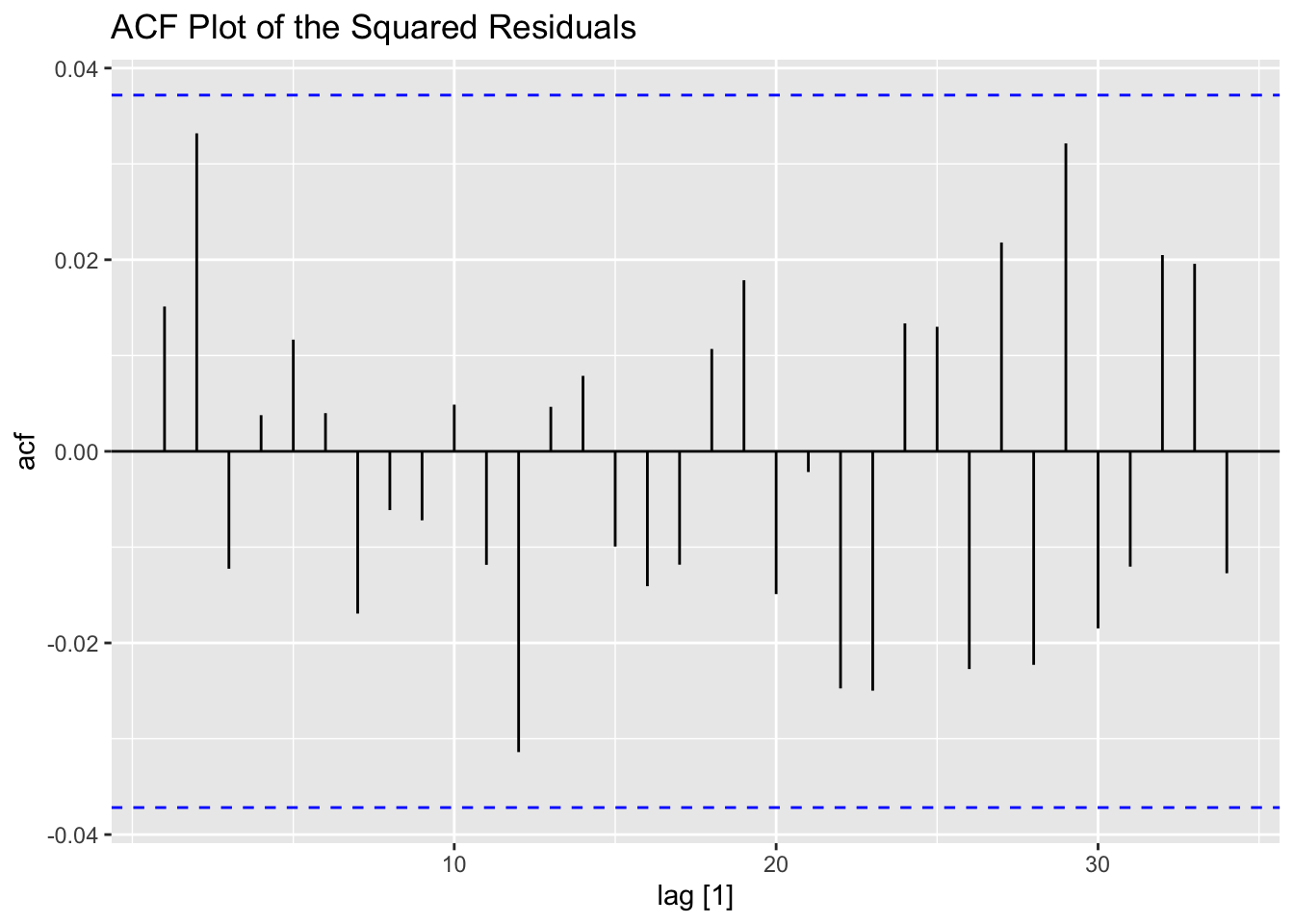

sp.garch.resid |>
  ACF(.resid^2) |>
  autoplot() +
  labs(title = "ACF Plot of the Squared Residuals")

6.2.2 Climate Series Example

For this example, we will be using the data from stemp.csv. This data contains monthly observations of temperature from 1850 to 2007 for the southern hemisphere. The data is from the database maintained by the University of East Anglia Climatic Research Unit. In the code chunk below, I read in the data, create an appropriate time variable, and declare the data as a tsibble.

(stemp <- read_csv("data/stemp.csv") |>
   pivot_longer(-year, names_to = "month", values_to = "anomaly") |>
   mutate(time = yearmonth(str_c(year, "-", month))) |>
   select(time, anomaly) |>
   as_tsibble(index = time))

## Rows: 158 Columns: 13
## ── Column specification ───────────────────────────────────────
## Delimiter: ","
## dbl (13): year, jan, feb, mar, apr, may, jun, jul, aug, sep, oct, nov, dec
## 
## ℹ Use `spec()` to retrieve the full column specification for this data.
## ℹ Specify the column types or set `show_col_types = FALSE` to quiet this message.

## # A tsibble: 1,896 x 2 [1M]
##        time anomaly
##       <mth>   <dbl>
##  1 1850 Jan  -0.625
##  2 1850 Feb  -0.598
##  3 1850 Mar  -0.841
##  4 1850 Apr  -0.632
##  5 1850 May  -0.326
##  6 1850 Jun  -0.528
##  7 1850 Jul  -0.296
##  8 1850 Aug  -0.503
##  9 1850 Sep  -0.602
## 10 1850 Oct  -0.42 
## # ℹ 1,886 more rows

As always the first step is to plot the new time series we are working with. The data appears to be very volatile at first glance. It also appears to have a slight upward trend over time.

stemp |> 
  ggplot(aes(x = time, y = anomaly)) +
  geom_point(size = 0.25) +
  geom_line() + 
  labs(title = "Plot of Temperature Anomaly over Time")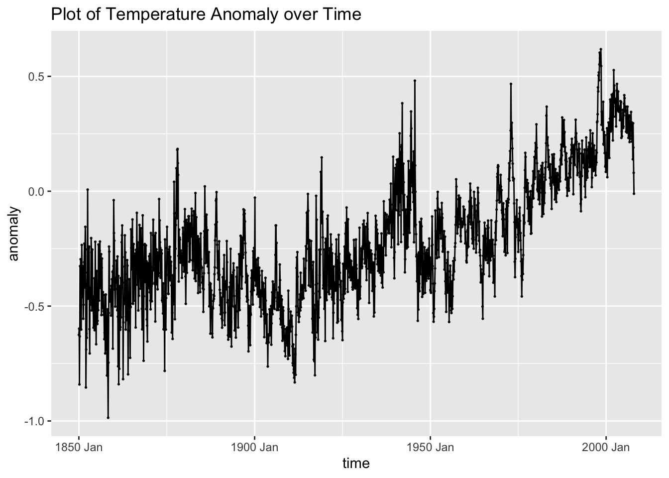

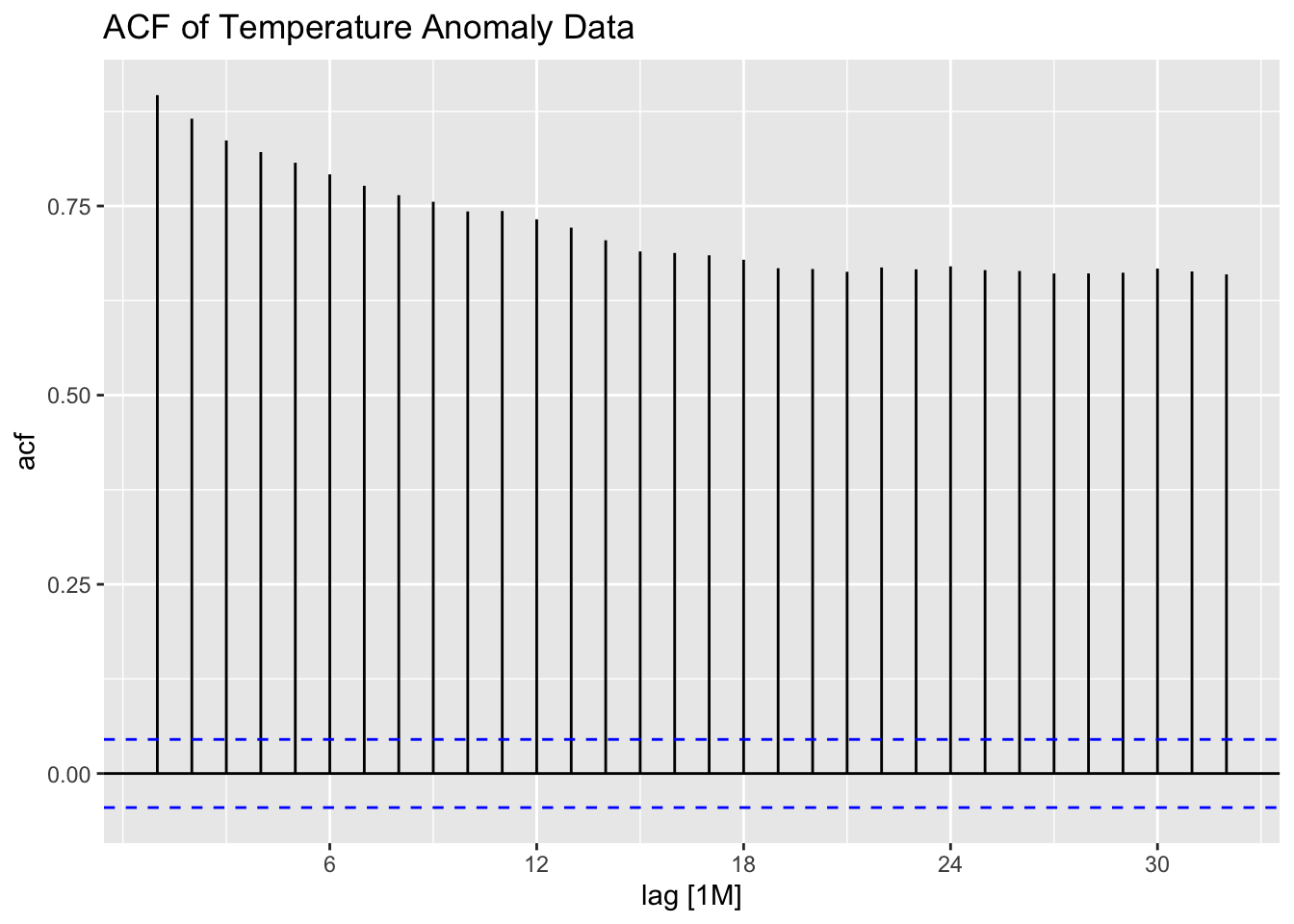
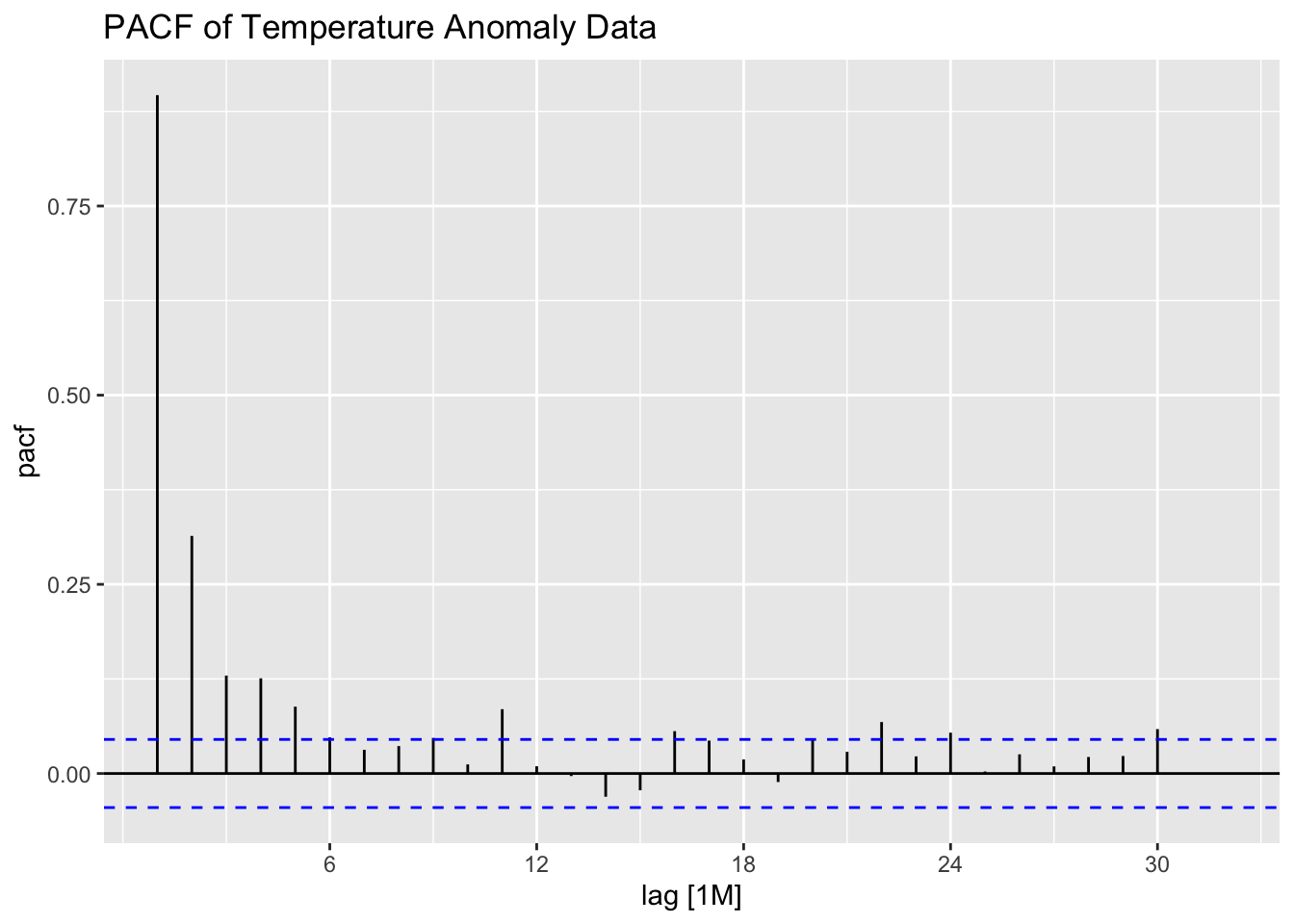
Examining the ACF and PACF of the data, it appears to have very high levels of lingering autocorrelation. This suggests that the data could benefit from differencing.

stemp |>
  ACF(anomaly) |>
  autoplot() +
  labs(title = "ACF of Temperature Anomaly Data")

stemp |>
  PACF(anomaly) |>
  autoplot() + 
  labs(title = "PACF of Temperature Anomaly Data")

The ACF and PACF of the first differenced series appear to be better than the untreated series, but still show lingering levels of autocorrelation. This suggests that second differencing may improve the ACF and PACF.

stemp |>
  ACF(difference(anomaly)) |>
  autoplot() + 
  labs(title = "ACF Plot of the First Differenced Temperature Anomaly Data")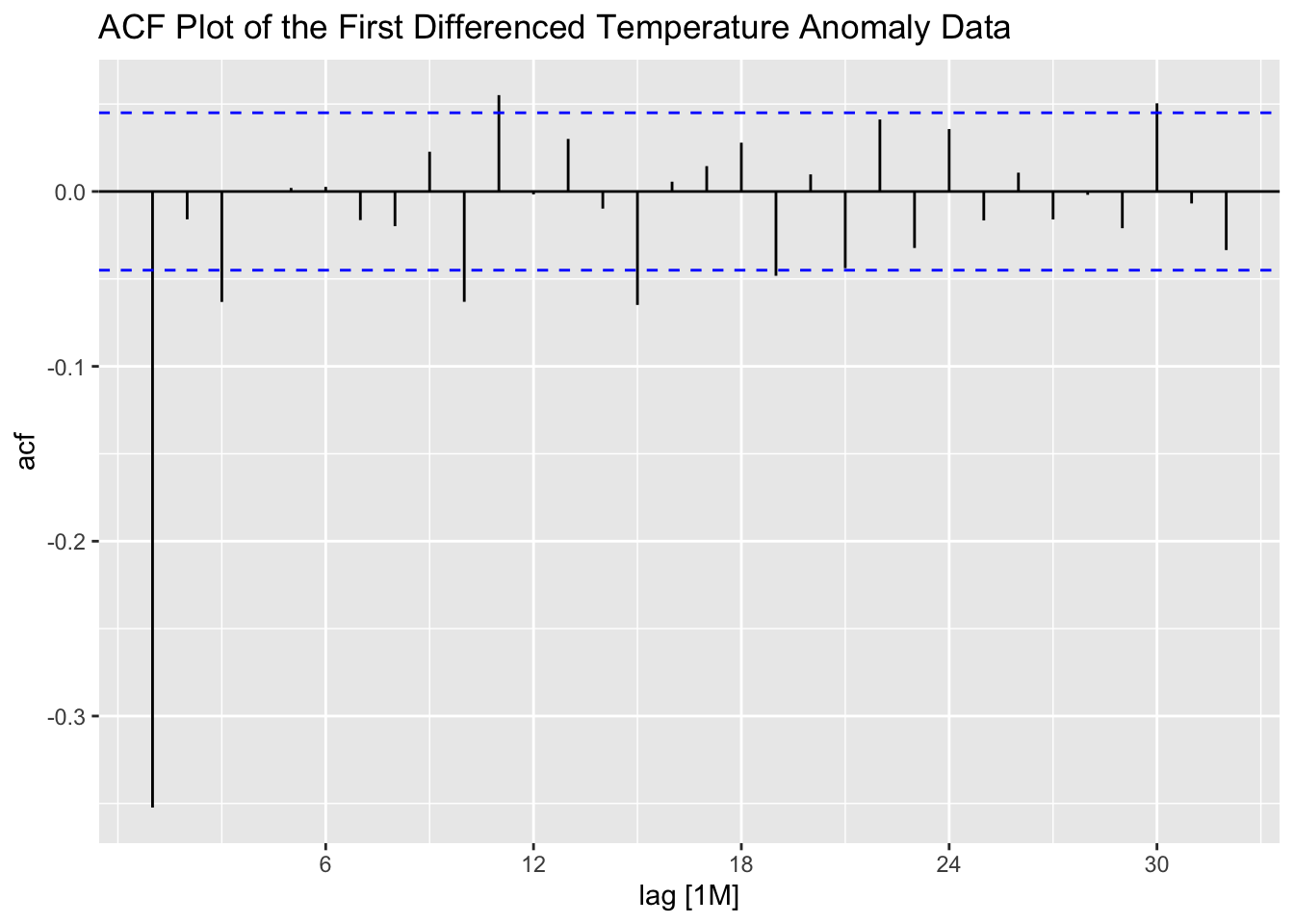

stemp |>
  PACF(difference(anomaly)) |>
  autoplot() + 
  labs(title = "PACF Plot of the First Differenced Temperature Anomaly Data")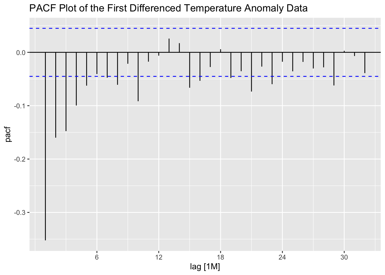

Second differencing the data appears to lead to a higher level of autocorrelation shown in the PACF, suggesting that simply first differencing the data is the best option.

stemp |>
  ACF(difference(difference(anomaly, lag = 1), lag = 1)) |>
  autoplot() + 
  labs(title = "ACF Plot of the Seconcd Differenced Temperature Anomaly Data")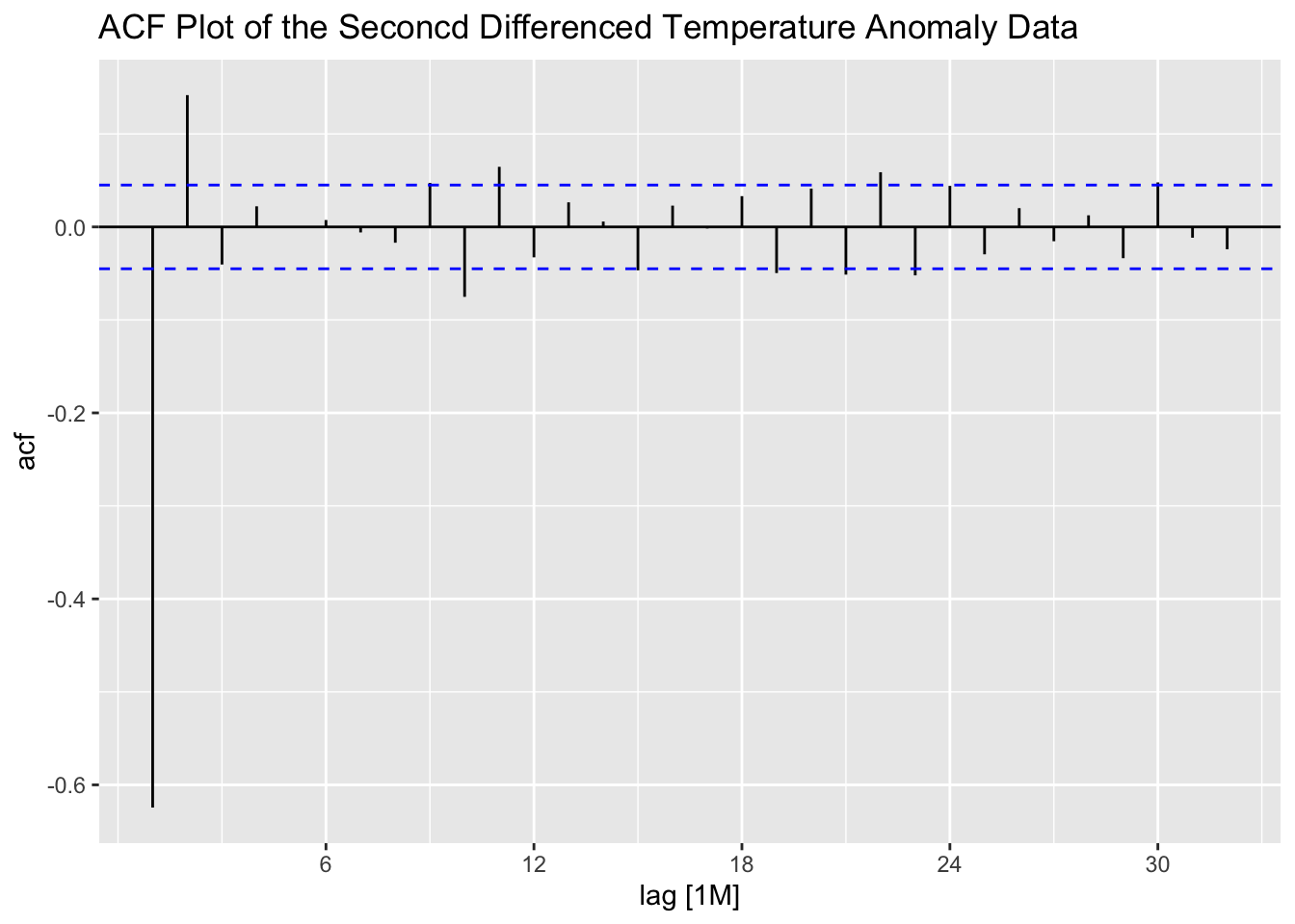

stemp |>
  PACF(difference(difference(anomaly, lag = 1), lag = 1)) |>
  autoplot() + 
  labs(title = "PACF Plot of the Second Differenced Temperature Anomaly Data")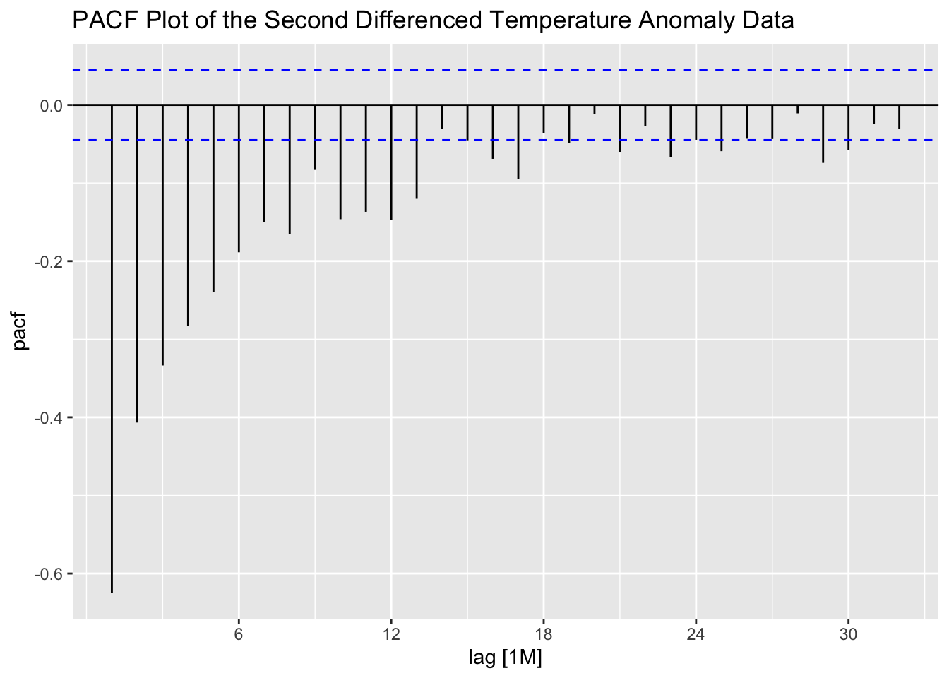

The next step is to fit an ARIMA model to the data. Below, I create a model object that contains an ARIMA(3,1,1)(2,0,0)[12] model, an ARIMA(1,1,2)(2,0,1)[12] model, and an ARIMA(1,1,2)(1,0,1)[12] model. The first model was selected as the best model by the ARIMA function through minimizing the AICc.

stemp.fit <- stemp |>
  model(arima_311_200 = ARIMA(anomaly, stepwise = FALSE),
        arima_112_201 = ARIMA(anomaly ~ 0 + pdq(1,1,2) + PDQ(2,0,1)),
        arima_112_101 = ARIMA(anomaly ~ 0 + pdq(1,1,2) + PDQ(1,0,1)))

Looking at the coefficients and their significance levels, the ARIMA(1,1,2)(1,0,1) model is the only model in which all coefficients are statistically significant. The ARIMA(3,1,1)(2,0,0) model has the lowest AICc, as expected, but performs slightly worse than the other models in measures of accuracy. The ARIMA(1,1,2)(1,0,1) model as the best one, as its measures of accuracy are close the others but all of its coefficients are significant.

stemp.fit |> tidy() |> mutate_if(is.numeric, dig) |> gt()

.model	term	estimate	std.error	statistic	p.value
arima_311_200	ar1	0.491	0.024	20.347	0.000
arima_311_200	ar2	0.183	0.026	7.119	0.000
arima_311_200	ar3	0.066	0.024	2.772	0.006
arima_311_200	ma1	-0.978	0.007	-136.565	0.000
arima_311_200	sar1	0.039	0.024	1.644	0.100
arima_311_200	sar2	0.026	0.024	1.092	0.275
arima_311_200	constant	0.000	0.000	1.715	0.087
arima_112_201	ar1	0.872	0.021	42.184	0.000
arima_112_201	ma1	-1.380	0.034	-40.115	0.000
arima_112_201	ma2	0.389	0.032	11.982	0.000
arima_112_201	sar1	0.931	0.037	24.915	0.000
arima_112_201	sar2	0.025	0.025	0.971	0.332
arima_112_201	sma1	-0.910	0.030	-30.136	0.000
arima_112_101	ar1	0.871	0.021	42.438	0.000
arima_112_101	ma1	-1.378	0.034	-40.370	0.000
arima_112_101	ma2	0.388	0.032	11.997	0.000
arima_112_101	sar1	0.960	0.018	52.770	0.000
arima_112_101	sma1	-0.919	0.026	-35.458	0.000

stemp.fit |> glance() |> select(-c(ar_roots, ma_roots)) |> mutate_if(is.numeric, dig) |> gt()

.model	sigma2	log_lik	AIC	AICc	BIC
arima_311_200	0.012	1500.008	-2984.016	-2983.940	-2939.640
arima_112_201	0.012	1518.600	-3023.200	-3023.140	-2984.371
arima_112_101	0.012	1518.107	-3024.213	-3024.169	-2990.932

stemp.fit |> accuracy() |> mutate_if(is.numeric, dig) |> gt()

.model	.type	ME	RMSE	MAE	MPE	MAPE	MASE	RMSSE	ACF1
arima_311_200	Training	0.000	0.110	0.083	Inf	Inf	0.556	0.566	-0.005
arima_112_201	Training	0.003	0.108	0.082	Inf	Inf	0.550	0.560	0.009
arima_112_101	Training	0.003	0.109	0.082	Inf	Inf	0.550	0.560	0.007

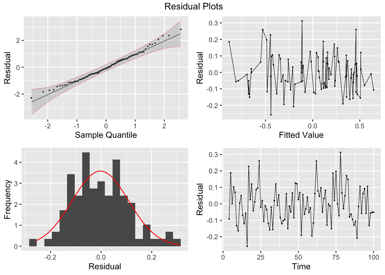
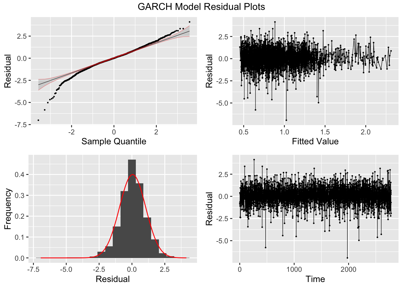
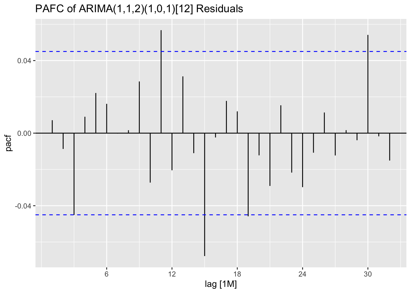
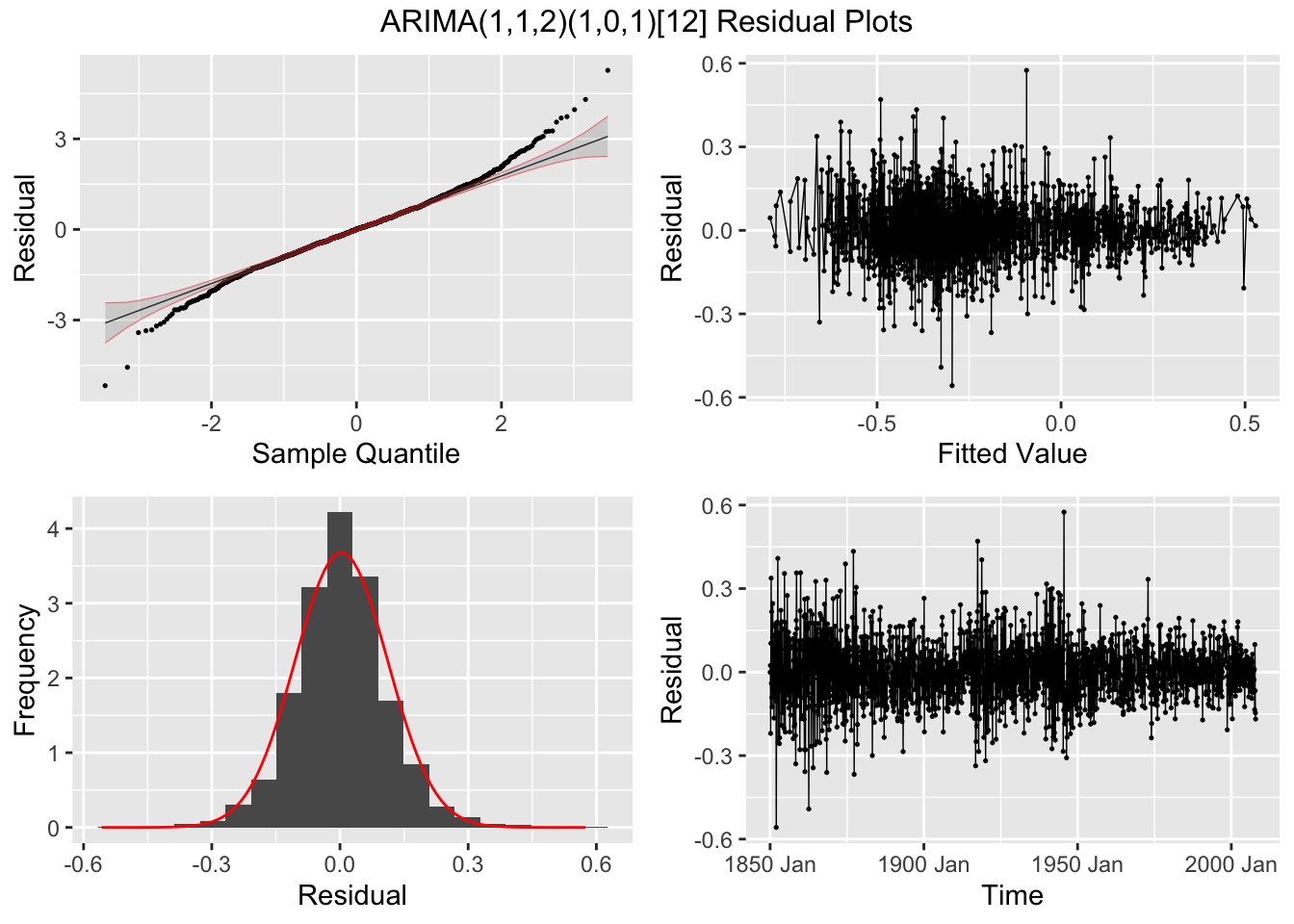
In the code chunk below, I use plot_residuals() to analyze the residuals of the ARIMA(1,1,2)(1,0,1) model. I additionally plot the ACF of the squared residuals. There appears to be lingering autocorrelation shown in all ACF and PACF plots, as well as the results of the Ljung-Box test.

stemp.fit |> select(arima_112_101) |>
  augment() |>
  plot_residuals(title = "ARIMA(1,1,2)(1,0,1)[12]")

## # A tibble: 1 × 3
##   .model        lb_stat lb_pvalue
##   <chr>           <dbl>     <dbl>
## 1 arima_112_101  0.0966     0.756
## # A tibble: 1 × 3
##   .model        kpss_stat kpss_pvalue
##   <chr>             <dbl>       <dbl>
## 1 arima_112_101    0.0817         0.1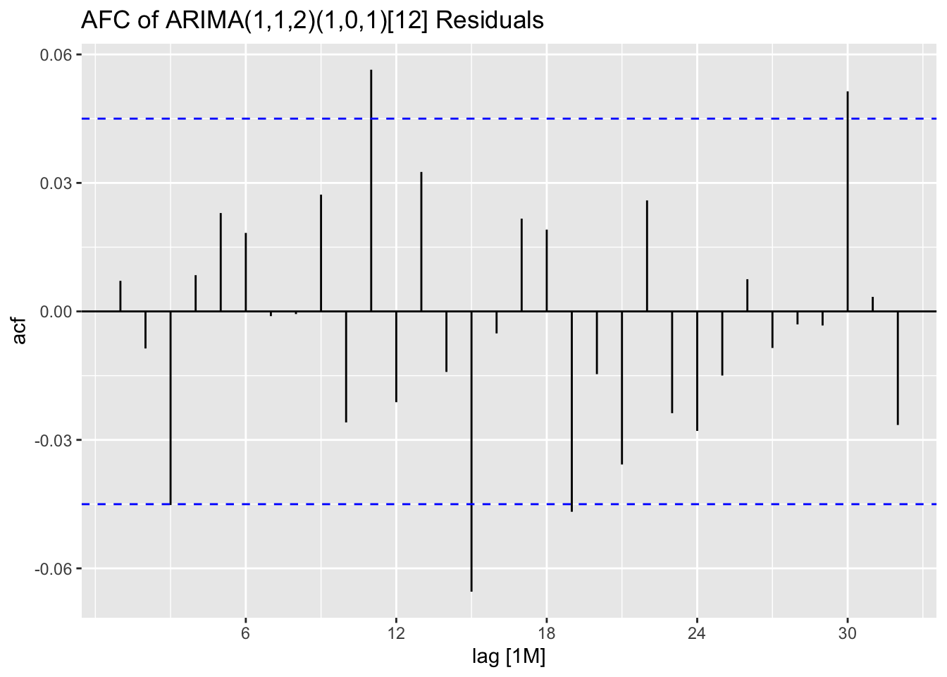

## NULL

stemp.fit |> select(arima_112_101) |>
  augment() |>
  ACF(.resid^2) |> autoplot()

To extract the signal remaining in the residuals, we will model the residuals from the ARIMA(1,1,2)(1,0,1) model using a GARCH model. I extract the residuals using augment(), isolate the residuals from the correct model and time variable using select(), and then declare the residuals as a time series. I use that time series with garch() to model the residuals. After creating a tsibble with the residuals from the GARCH model, I then plot the ACF of the residuals as well as the ACF of the squared residuals.

(stemp.resid <- stemp.fit |> select(arima_112_101) |>
  augment() |>
  select(time, .resid) |>
   as.ts())

##                Jan           Feb           Mar           Apr           May
## 1850 -6.249996e-04  2.371139e-02 -2.202986e-01  1.034806e-01  3.376496e-01
## 1851 -7.921286e-02  1.075650e-01  3.562421e-02 -1.651901e-01 -2.575468e-02
## 1852 -5.579254e-01 -1.049315e-01  2.135839e-02 -2.368521e-02  1.796631e-01
## 1853 -2.569663e-01 -2.360036e-01  1.754709e-01  2.204964e-02 -3.953763e-02
## 1854  5.607779e-03  2.179731e-02 -1.298934e-01  2.208230e-03 -8.327914e-02
## 1855  1.780979e-01  1.467217e-01 -8.218697e-02 -1.075665e-01 -6.055371e-02
## 1856  1.434646e-01 -1.286283e-01  6.662866e-03 -5.156824e-05  1.093022e-01
## 1857 -4.136388e-02 -4.220435e-02 -1.914767e-02 -1.175166e-01 -6.138619e-02
## 1858 -1.862869e-01  4.429881e-02  1.370896e-01 -2.278466e-01 -3.297510e-01
## 1859  2.784932e-02  4.553710e-02 -8.563235e-02  1.118908e-01 -4.303167e-02
## 1860  8.122025e-02  2.524295e-02 -1.675112e-01 -4.604969e-02 -9.227408e-02
## 1861  2.000339e-01 -1.695098e-01 -2.788304e-01  2.620318e-01 -3.576378e-01
## 1862 -6.963887e-02  9.638652e-02  2.652503e-01  1.599423e-01  1.566090e-01
## 1863  1.762760e-01  2.198194e-01 -3.979609e-02  8.500173e-02 -2.661335e-01
## 1864 -3.438521e-01  8.104439e-03  1.150818e-01 -2.381428e-02  1.751537e-01
## 1865 -4.435529e-03  4.874601e-02  1.396614e-01  1.550468e-01 -2.494128e-01
## 1866  1.183223e-01  5.911248e-03 -2.540134e-01  2.098659e-01  1.078431e-01
## 1867  1.500935e-01 -9.471380e-02  1.418054e-01  1.887801e-01 -2.187303e-02
## 1868 -1.587959e-01  1.454043e-01  3.300097e-01 -2.411915e-01  3.772227e-02
## 1869 -1.995598e-02  1.384398e-01 -2.074191e-01  1.022945e-01 -1.777391e-01
## 1870  1.426754e-01 -5.754211e-02 -6.274399e-02  1.199588e-01 -1.084536e-01
## 1871  8.088448e-02  1.648521e-01  1.645798e-01 -1.454833e-01 -1.586277e-02
## 1872  1.331942e-02  6.244337e-02 -1.079777e-01  3.429407e-02  1.020076e-01
## 1873  1.498924e-01 -2.886582e-02 -1.007057e-02 -1.368092e-01  6.491256e-02
## 1874  7.989006e-02 -1.885477e-01  5.150816e-02 -4.069838e-02 -8.814192e-02
## 1875  1.611447e-01  1.650289e-01 -5.909015e-02  2.082598e-02  4.754691e-02
## 1876  5.837252e-02 -2.728638e-02  1.320205e-02  1.988623e-02 -6.511381e-02
## 1877  8.641659e-02  4.336289e-01  8.865378e-02  3.100710e-02 -3.674392e-01
## 1878  3.046559e-01  1.599545e-01  7.110498e-02  2.019147e-02 -2.594228e-01
## 1879  1.176679e-02 -3.998623e-02 -1.088497e-02 -8.917120e-03 -3.820704e-02
## 1880  3.733262e-02  1.099930e-01  1.261094e-01 -6.412889e-02 -1.276212e-01
## 1881 -4.190029e-02 -2.761595e-02  1.068071e-01  4.967381e-02  1.007173e-01
## 1882  4.000605e-02  6.996134e-02  2.039962e-02 -4.565433e-02 -8.696748e-02
## 1883  1.790134e-01  6.539370e-02  1.378944e-01 -2.999864e-01 -7.774711e-03
## 1884 -3.855052e-02  6.965658e-02  5.451837e-02  3.280070e-03 -7.384592e-02
## 1885 -4.844375e-02 -1.175170e-01 -4.084322e-02 -6.287113e-02  3.685440e-02
## 1886 -7.617996e-02 -1.706227e-01  4.224460e-02  7.874914e-02  1.365448e-01
## 1887  3.872333e-02 -2.344524e-01 -3.384376e-02 -7.561455e-03 -6.036120e-02
## 1888 -1.298134e-01  3.877978e-02 -2.324675e-02  1.259235e-02  4.626008e-02
## 1889  1.639552e-01  9.620590e-02  9.055712e-02 -4.869316e-02 -6.892078e-02
## 1890 -1.154635e-01 -1.253736e-01 -1.416234e-01 -1.051391e-02 -8.077609e-02
## 1891 -4.630353e-02  9.268394e-03  6.217763e-02 -1.196781e-03  1.247560e-01
## 1892  8.751422e-03  1.656858e-01 -2.048931e-02 -1.665092e-01 -4.495348e-02
## 1893  6.357985e-02  6.006371e-02  1.629736e-01 -2.855818e-01 -5.480710e-02
## 1894  4.194697e-02 -1.802139e-02 -1.249750e-01 -7.447634e-02 -1.230405e-01
## 1895  8.219851e-02 -5.347158e-02 -4.390440e-02 -8.102773e-02 -9.179090e-02
## 1896  1.709040e-01  8.265198e-02  3.203216e-02  1.857852e-02 -1.120857e-01
## 1897 -6.329920e-02  1.148501e-01  5.953913e-02  5.190563e-02 -1.854901e-02
## 1898  5.114275e-02 -9.801834e-02 -1.673614e-01 -1.738488e-01 -1.699050e-02
## 1899  5.956778e-02  7.055838e-02  6.410520e-02 -4.153805e-02  5.598331e-02
## 1900  7.134536e-02  2.653211e-01 -2.147100e-01 -1.134437e-03 -4.570594e-02
## 1901  4.495628e-02 -5.725067e-02 -1.080992e-01  8.535455e-03  1.165353e-01
## 1902 -2.891143e-02  7.463185e-02  1.177447e-03  2.350353e-02  9.149189e-03
## 1903 -7.232041e-02  7.829613e-02 -4.873927e-02 -1.026826e-01 -1.071566e-02
## 1904 -6.144870e-02 -3.589680e-02 -1.724163e-02  1.085720e-01 -6.311186e-02
## 1905  6.230036e-02 -8.822965e-02  1.169104e-01 -1.095406e-02  5.342690e-02
## 1906  1.970998e-01  9.810147e-02 -7.461635e-02  9.135496e-02 -2.152623e-01
## 1907  4.477037e-02 -2.485716e-02  1.354446e-01  1.587757e-02 -1.297163e-01
## 1908  2.987708e-02  9.598764e-03 -7.885264e-03 -1.113465e-01  1.673755e-02
## 1909 -7.934089e-02 -2.553668e-02 -3.684033e-02  3.938886e-02 -4.887661e-02
## 1910  6.491936e-02 -3.949567e-02 -1.647713e-02  8.579084e-02  2.032004e-02
## 1911  4.060137e-03 -1.459869e-01 -6.293766e-02 -7.632453e-02 -2.112153e-02
## 1912  1.399990e-01 -2.670032e-02  1.489672e-01 -1.502891e-03 -1.102360e-01
## 1913 -6.622143e-02  1.414202e-01 -7.132251e-02  6.687187e-02  3.754848e-02
## 1914  1.462814e-01  1.495706e-02  3.167940e-02  1.158580e-02  1.259528e-02
## 1915  4.662394e-02  1.404513e-01  1.828644e-01  6.316100e-02 -7.136134e-02
## 1916  1.068561e-02  1.258955e-01 -2.946139e-02 -3.403526e-02  4.436361e-02
## 1917 -2.497213e-01 -5.160462e-02 -1.944048e-01  1.802504e-01 -3.144897e-02
## 1918 -7.068051e-02 -1.681418e-01  7.384457e-02 -3.118549e-02  1.191859e-01
## 1919  5.592780e-02  2.857524e-01 -1.040330e-01  4.065560e-02  7.746119e-02
## 1920 -2.796492e-02 -3.185418e-01  2.867765e-01  1.497166e-01  7.043184e-02
## 1921 -2.094557e-01  1.199530e-02 -7.039814e-02 -7.307100e-02  1.487162e-01
## 1922 -1.447568e-01  1.151564e-01 -1.464040e-01  4.461786e-02 -2.536537e-01
## 1923 -2.947838e-02  1.263757e-01  2.283800e-02  1.206293e-01 -1.331560e-01
## 1924 -9.139755e-02  5.274683e-02  1.715600e-03 -4.330634e-02 -3.953788e-02
## 1925 -9.967925e-02  7.167582e-02  1.942593e-01 -5.481715e-02 -1.907535e-02
## 1926 -2.556010e-03 -1.067355e-01  2.296154e-01  1.336020e-02 -3.873923e-02
## 1927 -3.774797e-02  6.108594e-02 -7.299850e-02  4.472702e-02  5.214471e-03
## 1928  8.182184e-02  5.604415e-03 -8.174759e-02  1.677612e-01 -9.482776e-02
## 1929 -2.363578e-02 -1.041314e-01 -1.463695e-01  3.729000e-02 -1.070043e-01
## 1930 -8.524442e-02 -1.019898e-02  1.001029e-01  2.002179e-02  1.214790e-01
## 1931  1.063850e-01  7.502561e-02  2.705241e-02 -6.726931e-02 -5.659143e-02
## 1932  1.849207e-01  5.299542e-02  1.083643e-01 -6.076868e-02 -4.307535e-02
## 1933 -3.110031e-04  1.826462e-02 -8.665483e-02 -9.496771e-03  7.521822e-02
## 1934  1.345911e-01 -1.732988e-01  2.192779e-02  1.336339e-01  6.570544e-02
## 1935  8.376989e-02 -8.160678e-02 -7.615640e-02  2.159907e-02  6.515996e-02
## 1936 -2.317305e-02  1.365620e-01 -1.496245e-01 -1.261522e-02  4.364158e-03
## 1937  5.973185e-02  1.009118e-01 -4.999674e-02  4.050270e-03 -5.829345e-02
## 1938 -2.620107e-02  4.296165e-03  8.136835e-02  3.051147e-02 -1.491622e-02
## 1939  8.925684e-02 -5.928371e-04 -4.596903e-02  9.129230e-02  1.029921e-01
## 1940  2.056866e-01  8.751959e-03 -4.592472e-02  9.171733e-02  1.691688e-01
## 1941 -9.642091e-02 -4.737907e-02  9.940653e-02  2.956864e-01 -1.235091e-01
## 1942  2.632867e-01 -2.333566e-01  6.079031e-03 -1.570908e-01  1.658734e-01
## 1943  9.578738e-02 -7.742049e-02 -3.284294e-03 -1.040964e-01  3.063027e-02
## 1944 -4.937488e-02 -8.810785e-02  2.295232e-01  3.050028e-02 -6.847483e-02
## 1945 -8.995094e-02  5.539268e-02 -8.054958e-02  1.793397e-01 -2.849512e-01
## 1946 -1.793138e-01 -7.484479e-02 -1.757303e-01 -3.834464e-02 -6.580422e-02
## 1947  2.042987e-01 -5.440040e-02 -1.223985e-01  7.197575e-02 -2.742982e-02
## 1948 -1.218209e-01  1.025678e-02  4.475837e-02 -9.932127e-02  9.857656e-02
## 1949  5.722177e-02 -8.516525e-02  3.751959e-03  9.149384e-03 -3.156818e-02
## 1950 -1.546900e-01 -7.408904e-02 -6.231232e-02  3.158441e-02  3.888996e-02
## 1951 -8.627690e-02 -1.840051e-02  3.949847e-02  6.288285e-03  6.835902e-02
## 1952  2.175725e-01  1.547667e-01  1.607728e-02 -8.308257e-02 -4.119636e-02
## 1953 -4.475623e-02  7.301298e-02  5.649036e-02  8.218687e-02  1.876215e-02
## 1954 -1.581160e-01  2.268796e-02  5.700315e-02 -1.866339e-01 -1.323741e-01
## 1955  9.359611e-02 -7.144624e-02 -9.449160e-02 -5.172556e-02 -1.811709e-01
## 1956 -8.375771e-02  7.950043e-02  2.331317e-02 -1.307542e-01 -1.659800e-05
## 1957  5.634765e-02  4.755418e-02  1.070659e-01  9.251789e-02  2.392751e-01
## 1958  1.186373e-01  9.105694e-02 -4.263218e-02  1.526326e-02  2.872642e-02
## 1959  9.506900e-03  1.025415e-02  3.097131e-02  2.504381e-02  1.768864e-02
## 1960  5.872587e-03 -4.152164e-02 -1.864644e-02 -8.883959e-02 -4.297514e-02
## 1961  1.354287e-02  1.059975e-01 -9.115784e-03  7.962862e-02  1.342778e-01
## 1962 -6.052076e-02  6.134622e-02  1.860364e-02 -4.309570e-02 -6.289143e-02
## 1963 -1.104630e-01 -2.154454e-02  4.427655e-02 -4.283694e-04  1.348738e-01
## 1964 -1.176648e-01 -5.206738e-02 -5.494254e-02 -7.877284e-02 -1.207509e-01
## 1965  1.749331e-01  1.407399e-01 -1.079686e-01  1.117762e-02  4.585050e-02
## 1966  3.983521e-03 -5.476927e-02 -1.370279e-02  1.115185e-01 -1.089150e-01
## 1967 -3.862753e-02 -5.879149e-02 -1.030958e-02  5.049124e-04  1.438806e-01
## 1968  2.231957e-02 -9.984459e-02  7.264032e-03 -2.381784e-02 -1.352469e-01
## 1969  1.563005e-01  1.093426e-01  1.092457e-01  8.412182e-02  7.212404e-02
## 1970  7.853078e-02  7.564931e-03 -3.821027e-02  4.366026e-02 -4.557635e-02
## 1971 -5.844479e-02 -1.215200e-01 -4.944485e-02 -4.328167e-02  1.138305e-02
## 1972  1.284484e-01  9.715540e-02  3.911593e-02  3.527299e-02  1.230144e-01
## 1973 -1.687933e-02  7.821661e-04  1.074664e-01  1.203717e-02  5.526499e-04
## 1974 -2.364189e-01 -1.843833e-01 -2.741168e-02  5.387651e-02  9.818013e-02
## 1975 -1.157249e-01 -9.397455e-03  3.865690e-02  1.672336e-02  4.244341e-02
## 1976 -1.673141e-01  2.653930e-02 -7.466035e-02  2.260092e-02 -7.763452e-02
## 1977  1.703232e-01  8.243653e-02 -4.775965e-02 -5.246640e-02  3.290841e-02
## 1978  2.444771e-02  3.960984e-02  3.342934e-02 -1.032421e-01  5.577476e-02
## 1979  1.003157e-01  1.216353e-02  5.915379e-02  9.343763e-02 -6.633059e-02
## 1980  8.404468e-03  8.459836e-02  1.516637e-01 -7.846218e-03 -4.337787e-02
## 1981 -1.486075e-02 -7.193875e-02  1.407090e-02  2.694061e-02  7.341756e-02
## 1982  2.615186e-02 -1.143873e-01 -9.336174e-02  2.678999e-02  7.311469e-02
## 1983  1.935245e-01  1.585049e-01 -4.046186e-02  4.724722e-03  3.144587e-02
## 1984 -4.470211e-02  4.623656e-02 -5.631218e-02 -3.536251e-02 -1.241158e-04
## 1985  5.074335e-02  6.759367e-02  6.051201e-02 -9.956362e-02 -4.193566e-03
## 1986 -4.640509e-02  6.114685e-02  2.570827e-02 -3.320791e-02 -3.070801e-02
## 1987  7.725397e-02  3.984371e-02  6.464138e-02  6.891663e-02 -4.624316e-02
## 1988  1.022134e-01  4.038549e-03  2.664136e-02 -5.341620e-02  6.628988e-03
## 1989 -1.192910e-02  1.325325e-02 -1.904195e-02 -1.855414e-02 -3.342977e-02
## 1990  3.582388e-02  4.737916e-02  5.133827e-02  6.294169e-02  8.006401e-03
## 1991 -3.607577e-02 -2.231227e-02  8.243783e-02  7.515596e-02  1.208122e-01
## 1992  2.598987e-02  4.040298e-02  3.044413e-02  4.705162e-02 -1.882628e-02
## 1993  1.657077e-01 -3.324111e-02  1.303300e-01 -3.468883e-02  7.784399e-03
## 1994 -2.541221e-03 -1.292123e-01  6.294435e-02 -3.881466e-02  1.588985e-01
## 1995  9.383361e-03  2.805561e-02  2.235994e-02 -8.188490e-02 -2.445676e-02
## 1996 -4.190306e-02  1.272278e-01  8.864076e-02 -6.201352e-03 -4.580800e-02
## 1997 -8.873274e-02  2.321499e-04  4.538524e-02 -1.980005e-02  2.650409e-02
## 1998  3.875825e-02  1.157894e-01  1.232532e-01  8.454677e-02  8.464362e-02
## 1999 -4.493537e-02 -1.704735e-02  9.758114e-02 -1.161277e-01 -6.239433e-02
## 2000  8.937883e-03  1.128038e-02 -5.538870e-02  1.222820e-01 -1.678103e-01
## 2001  8.279984e-02  7.380144e-02  1.038507e-01  6.035261e-02 -8.626234e-02
## 2002  1.610008e-01 -2.586906e-02  1.805887e-01  1.637873e-02  6.008624e-02
## 2003  9.658049e-02  8.118796e-02 -5.098901e-03 -8.447595e-03 -3.670827e-02
## 2004  1.727429e-02  4.093055e-02 -5.010691e-02  4.364773e-02 -1.243126e-01
## 2005  2.084444e-02  5.534056e-02  4.658341e-02  2.611046e-02 -2.618512e-02
## 2006  3.245425e-02  4.780635e-02 -4.100370e-02 -3.174253e-02 -6.967219e-02
## 2007 -8.369953e-03  3.615690e-02 -7.266677e-02  2.600826e-03 -7.078632e-02
##                Jun           Jul           Aug           Sep           Oct
## 1850 -4.024989e-02  2.166876e-01 -9.127531e-02 -1.250457e-01  1.271816e-01
## 1851  7.940774e-02  1.339840e-01  1.642194e-01 -8.919921e-02  9.824102e-02
## 1852  1.422036e-01  4.084533e-01 -2.522586e-01  4.423655e-02 -5.624302e-02
## 1853  2.074913e-02  2.219029e-01  8.170500e-02 -1.906773e-01 -6.811217e-02
## 1854  1.552527e-01 -2.013148e-01 -6.085440e-02  3.542865e-01 -8.648265e-02
## 1855  7.186104e-02 -7.201692e-02  2.750797e-01 -3.590133e-02 -8.072435e-02
## 1856 -2.149766e-01  8.458734e-02  9.496826e-02 -1.546619e-01 -3.681431e-02
## 1857  1.200098e-01 -2.391456e-01  4.141460e-02  1.178188e-01 -7.279007e-02
## 1858  4.463456e-02  1.859150e-01  3.562051e-01  1.564268e-01 -1.213665e-01
## 1859  8.175525e-02 -6.810731e-02  7.932474e-02 -2.788268e-01  2.201022e-01
## 1860  1.588160e-02  3.997235e-02 -7.726416e-04  1.132508e-01 -3.293896e-02
## 1861  2.064274e-01 -2.792672e-01  1.975381e-01  7.918018e-02 -1.299935e-01
## 1862 -7.583529e-02 -1.248615e-01 -4.918925e-01  2.698712e-02  1.175031e-01
## 1863 -9.382254e-02  1.091801e-01 -6.777547e-03 -1.185859e-01  2.074557e-01
## 1864 -1.401646e-01  5.120652e-02 -2.607884e-01  9.714672e-02  2.919877e-02
## 1865 -1.212890e-01  6.225331e-02  1.743461e-01 -1.527103e-01  7.680766e-02
## 1866  5.833198e-02  2.003137e-01 -8.592311e-02 -1.198865e-01  1.276859e-01
## 1867 -5.477135e-02 -3.946928e-02 -7.772912e-02  2.439225e-01  3.841807e-02
## 1868 -3.606322e-01  8.094215e-02  1.544383e-01  1.731163e-01  7.714114e-02
## 1869 -1.120077e-01 -1.624525e-01  1.521763e-01  1.547823e-01 -1.582161e-02
## 1870 -8.429975e-02  2.637893e-01 -8.817720e-02 -6.113866e-02 -1.020846e-01
## 1871  2.661622e-02  1.144111e-01 -1.355583e-01 -6.753168e-02 -1.975027e-01
## 1872 -1.027948e-01  3.942125e-02  6.355862e-02 -6.211058e-02 -1.092505e-02
## 1873 -2.204064e-02  5.073142e-02  2.407264e-02 -1.855369e-01 -7.632545e-02
## 1874 -2.478836e-01  3.887712e-01 -4.651205e-02 -2.458033e-02 -1.755027e-01
## 1875 -1.287798e-01 -1.177463e-01  9.240472e-02  1.125954e-01 -6.645977e-02
## 1876 -2.092278e-01 -6.190689e-03 -7.457060e-02 -1.572033e-01  1.963041e-01
## 1877  8.853945e-02  7.011146e-02  1.555179e-01  1.483640e-01  2.836180e-01
## 1878 -1.883756e-01  8.986965e-02 -3.608760e-02  5.584006e-02  1.772338e-02
## 1879  7.455057e-02  6.109829e-03  1.260488e-01  4.149022e-02 -1.144243e-01
## 1880 -1.581292e-01  1.319996e-04  2.228999e-01 -4.200102e-03 -1.136965e-01
## 1881 -1.148645e-01  4.501243e-02 -4.277388e-02 -7.687018e-02  1.246221e-01
## 1882 -5.240792e-02  1.398178e-02 -5.467794e-02  1.984270e-01 -7.278403e-02
## 1883  2.182772e-01 -8.611627e-02  1.323244e-04 -8.621570e-02 -9.221320e-02
## 1884 -6.763353e-02 -1.206379e-01  8.100660e-02  1.357145e-01 -4.483402e-02
## 1885 -1.181087e-01 -1.738674e-02  3.869778e-02  1.876518e-01  6.756782e-02
## 1886 -1.064071e-01 -8.940515e-02  8.985315e-02 -1.204934e-01 -2.018727e-02
## 1887 -1.627002e-01  7.769075e-02 -2.488527e-02 -2.946496e-02 -1.361022e-01
## 1888  1.910102e-02 -3.740637e-02  5.381646e-02  4.561488e-02  1.458580e-01
## 1889 -8.761068e-02 -2.699332e-03 -1.050501e-01 -7.796932e-02 -3.419917e-02
## 1890  2.750041e-02 -2.578595e-02 -4.968039e-02 -1.143914e-01 -1.057351e-01
## 1891 -1.651123e-01 -1.752218e-01 -4.852117e-02  9.004457e-02  4.421517e-02
## 1892 -1.471568e-01 -1.366272e-01 -9.169019e-03  2.612939e-02 -3.468440e-02
## 1893 -1.080217e-01  1.128084e-01  1.245748e-01 -8.619053e-02  7.894669e-02
## 1894  2.310949e-02  1.520720e-02 -2.291116e-02 -1.513470e-01  3.195084e-02
## 1895  1.650435e-01 -4.480350e-02  1.786640e-01 -9.757920e-02 -9.631195e-02
## 1896  3.447126e-02  9.554430e-02  1.000826e-01 -1.051702e-02  2.362709e-02
## 1897 -7.383386e-03 -1.475623e-01 -1.018000e-02 -1.719556e-02 -1.046470e-01
## 1898  1.257820e-01 -1.095367e-01  1.393442e-02  1.773936e-02 -1.628987e-01
## 1899  4.701765e-02 -9.470477e-02  1.612998e-01  6.670439e-02 -9.160995e-02
## 1900  2.930987e-02  8.460187e-02 -9.364655e-02  1.442824e-02 -5.903916e-02
## 1901  3.136529e-02 -1.324975e-01 -1.641313e-02 -1.974498e-02 -4.013409e-03
## 1902 -8.731117e-02  6.401417e-02 -1.326334e-01  2.086826e-02 -1.593993e-01
## 1903 -1.215057e-01  4.223028e-02 -1.337257e-01 -3.837475e-02 -1.546390e-01
## 1904  3.172469e-02  6.754145e-03 -1.457115e-02  3.893657e-02 -1.295963e-01
## 1905  1.672698e-02 -4.883427e-02  6.882655e-02 -6.813444e-02  4.943234e-02
## 1906 -3.872137e-02  1.206616e-02 -2.879688e-02 -3.536384e-02 -1.386999e-02
## 1907 -7.468956e-02 -1.215036e-02  5.873831e-02  1.116807e-02  3.485742e-02
## 1908 -4.932094e-02 -4.178471e-02 -1.071498e-01  9.824201e-03 -7.864639e-02
## 1909  1.738853e-02 -1.143344e-01  2.174397e-01  2.062413e-02 -1.108126e-01
## 1910 -6.926716e-03  3.245132e-02 -8.920592e-03 -4.390677e-02 -8.028919e-02
## 1911 -5.673980e-02  8.811586e-02 -2.181977e-02 -1.046954e-01  1.375864e-01
## 1912 -3.941066e-02 -9.742173e-03 -5.821751e-02  4.730803e-02  1.015662e-02
## 1913  2.670897e-02  7.218354e-02  1.521290e-04  2.518142e-02  1.973842e-02
## 1914  1.147629e-01 -4.143951e-02  1.766970e-01  4.657106e-02  1.142352e-01
## 1915 -1.546703e-01  1.050371e-01  7.953183e-02  2.843320e-03 -2.216007e-02
## 1916 -1.663080e-01 -1.515078e-01  1.278800e-01  1.477867e-01 -4.661283e-02
## 1917  2.173382e-01  4.702330e-01 -2.812887e-02  1.512316e-01 -1.605245e-01
## 1918  2.398300e-01 -1.691020e-02 -1.093791e-01  1.416915e-01  1.267710e-01
## 1919 -4.377069e-02 -2.347057e-01 -9.171578e-02  6.425210e-03 -9.575234e-03
## 1920  6.650369e-02 -2.166887e-01  7.606376e-02  2.044643e-01  4.887749e-02
## 1921  1.046448e-01 -1.264407e-03 -1.260744e-01  1.641813e-01  4.589121e-02
## 1922 -1.883079e-02  1.794065e-01 -9.440096e-02  1.632520e-02  2.905470e-03
## 1923  6.975970e-02 -2.411458e-01 -1.967963e-02 -1.282764e-01 -5.762094e-02
## 1924 -3.543617e-02 -6.838496e-02  3.805981e-02 -1.741748e-01  1.429512e-02
## 1925  7.389093e-02  5.780732e-02  1.327984e-01 -1.453766e-01 -2.421877e-02
## 1926  7.484170e-02 -1.927791e-01  2.197292e-01 -3.256867e-02  1.258902e-02
## 1927 -4.891122e-02  7.724876e-02 -2.939418e-02  8.662074e-03 -3.869286e-03
## 1928 -4.875963e-02  9.384280e-02  7.853664e-02 -1.296738e-01  8.555320e-02
## 1929  4.537128e-02 -1.172186e-01  7.304768e-02 -4.415631e-02  6.538232e-02
## 1930  3.785153e-02 -3.618813e-02 -2.988353e-02  3.507091e-02  8.228709e-02
## 1931  3.556463e-02  1.313777e-01 -7.925614e-02 -4.440655e-02 -3.056528e-02
## 1932 -8.303402e-02  5.715766e-02 -2.191862e-01  1.649875e-01 -4.810090e-02
## 1933 -3.287484e-02 -1.128165e-01  4.272747e-02 -1.656956e-02  4.452723e-02
## 1934  2.100806e-01  6.741681e-02  6.372680e-02  2.901743e-02 -7.092744e-02
## 1935  3.513982e-02 -6.947063e-03 -9.095178e-02  6.452807e-02 -1.063807e-02
## 1936 -9.490348e-02  1.323132e-01  5.226373e-02 -8.375051e-02  2.801749e-01
## 1937  5.826712e-02  8.757002e-02  8.199153e-02  2.556289e-02  3.080242e-02
## 1938  1.374884e-01 -1.950203e-02 -2.668382e-03  7.141165e-02  1.559598e-01
## 1939  2.517519e-01  2.370895e-02 -4.827212e-02 -2.404122e-01 -2.006662e-01
## 1940 -4.990824e-02  1.567650e-01 -3.183915e-03  1.112789e-01 -1.286527e-01
## 1941  1.634193e-01  9.171564e-02 -1.266889e-02 -2.754106e-01  3.003566e-01
## 1942 -1.560442e-02 -2.180566e-01  7.774896e-02 -9.473506e-02 -2.443157e-01
## 1943  4.056770e-02  1.161234e-01 -1.685446e-01  3.201939e-02  2.849409e-01
## 1944  2.757409e-01  2.567996e-01  8.129787e-02 -6.318264e-02 -1.021358e-01
## 1945  8.051711e-02 -1.362367e-01  5.747660e-01 -6.248186e-02 -1.301527e-01
## 1946 -3.080659e-01  1.091399e-01 -2.344076e-01  1.330093e-01  3.008461e-02
## 1947  9.117808e-02 -3.177103e-03 -1.708404e-01 -2.214931e-01 -8.887567e-02
## 1948 -2.994174e-02 -1.995144e-01 -2.263522e-02 -2.483107e-02  6.365134e-02
## 1949 -1.181376e-01  6.565678e-02 -5.407232e-02  9.837738e-02 -1.332113e-01
## 1950  6.362904e-02  1.486299e-01 -5.436743e-02 -9.962115e-02 -1.291525e-01
## 1951  2.456406e-01  1.812758e-02 -1.278494e-03 -5.653283e-02  4.845589e-02
## 1952 -1.359487e-01  8.058290e-02  5.973547e-02  1.040496e-01  2.727672e-04
## 1953 -2.099334e-02 -1.528834e-01 -3.917983e-02  4.260250e-02 -2.378874e-02
## 1954 -9.265790e-02 -1.506376e-01  7.329094e-02 -1.116946e-02  6.542486e-02
## 1955  1.900242e-02 -8.757813e-02  8.383666e-02  6.250834e-02 -1.359246e-01
## 1956  4.818114e-02  7.789605e-02 -6.078138e-02  1.899343e-02  6.480839e-04
## 1957  7.632377e-02 -9.860122e-02  4.036322e-02 -5.918274e-02  2.671231e-02
## 1958 -3.190613e-02  1.227021e-01 -1.004962e-01 -4.580265e-02  8.853175e-02
## 1959  7.408184e-02 -2.676965e-02  2.290743e-02  9.254342e-03  7.528760e-02
## 1960 -1.790419e-02  2.317835e-02  8.102364e-02  1.084689e-01  3.819166e-03
## 1961  3.061482e-02 -1.087537e-01  7.268667e-02  1.303359e-02  2.567859e-02
## 1962  1.966827e-01  6.372351e-03 -8.240789e-03  9.445646e-02  2.354925e-04
## 1963 -3.237008e-03  1.375409e-01  4.578198e-02 -3.608510e-03 -7.019570e-02
## 1964 -3.928532e-02 -4.866232e-02 -6.504040e-02 -5.367153e-02 -1.165632e-02
## 1965  9.794816e-02 -1.010616e-01  5.630887e-02  4.828682e-02 -1.695091e-02
## 1966  1.041916e-01  3.134914e-02 -1.358595e-01 -1.368445e-02 -1.193872e-01
## 1967 -9.737450e-02 -4.965197e-02 -3.309224e-02 -3.700664e-03  5.780786e-02
## 1968  1.240014e-01  1.117395e-01  9.315834e-02 -2.713849e-02  7.955656e-02
## 1969 -6.725324e-02 -3.840860e-02  5.216881e-02 -1.499781e-02  7.044915e-02
## 1970 -4.352690e-02 -2.821064e-02 -8.763575e-02  6.861128e-02  7.578077e-02
## 1971 -7.412428e-02  1.677450e-01  2.925888e-02  9.684127e-02 -4.494118e-02
## 1972  1.232397e-01  4.188508e-03  7.755130e-02  1.303324e-01  4.399600e-02
## 1973 -5.429159e-02 -5.533086e-02 -2.342992e-02  6.237108e-03  1.876382e-02
## 1974  1.994120e-02  1.110035e-02  6.835880e-02 -8.083922e-02 -5.082272e-02
## 1975  2.723247e-02 -4.073074e-02 -1.118331e-01 -2.617694e-02 -9.233588e-02
## 1976  9.346337e-03  1.652048e-01 -2.291290e-02  3.328561e-02  2.167044e-02
## 1977  9.579460e-03  3.468152e-02 -4.166398e-02 -6.053121e-02  9.272998e-02
## 1978 -2.106792e-02  6.569712e-02 -1.450831e-01  6.129636e-02 -1.008679e-01
## 1979  3.109767e-02  5.227924e-02  1.316154e-01 -2.403339e-02  1.704399e-02
## 1980 -1.286511e-01 -4.568834e-02 -1.942417e-02  1.151922e-02 -3.836124e-02
## 1981  2.628171e-02  4.487311e-02  5.322460e-02 -6.248086e-03 -1.680299e-01
## 1982 -6.495215e-02  8.357515e-03  7.666966e-02  7.784363e-02  4.561605e-03
## 1983 -2.352240e-03 -8.223200e-02  5.247958e-02  5.623029e-03 -1.414840e-02
## 1984 -3.405294e-02 -1.082420e-01  7.952459e-02  1.313643e-01 -3.519801e-02
## 1985 -1.050046e-01  5.569098e-02  4.407335e-02 -6.556151e-02  4.066762e-02
## 1986  2.371422e-02 -1.659396e-03 -4.628878e-02  3.814113e-02  6.850794e-02
## 1987  2.935593e-02  1.847106e-01 -2.565764e-02  1.995145e-02  5.823906e-02
## 1988 -4.296374e-02 -1.058985e-01  4.184277e-02  4.176724e-02 -3.513315e-03
## 1989 -3.036303e-02  4.728606e-02  7.921469e-02 -5.456818e-04 -5.349941e-03
## 1990 -1.515582e-02  1.149274e-02 -2.554006e-02 -1.719984e-01  1.403662e-01
## 1991  1.549245e-02  1.259498e-02 -2.146322e-02 -2.793590e-02 -8.053579e-02
## 1992  2.232329e-02 -1.147639e-01 -3.406283e-02 -6.886651e-02 -1.205749e-01
## 1993  2.414780e-02 -2.152630e-02 -1.242335e-02  1.131552e-02 -2.153803e-02
## 1994  1.976605e-02 -6.221078e-02 -6.428207e-02 -3.485344e-02  1.430678e-02
## 1995  3.107675e-02  1.210185e-01 -2.823330e-02 -6.497870e-02 -2.807174e-02
## 1996 -7.434782e-02  2.469800e-02  6.226668e-02 -6.605953e-02  1.793833e-02
## 1997  1.504190e-01  7.695023e-02  7.950729e-02  1.807822e-01  9.171884e-02
## 1998  3.962534e-02  1.130559e-01  1.623043e-02 -2.074862e-01 -1.360990e-02
## 1999  2.686018e-02 -1.100053e-02 -7.986208e-02  5.220467e-02 -1.147160e-01
## 2000  4.800136e-02 -4.337737e-02  4.959726e-02  1.093672e-01 -4.322969e-02
## 2001  8.555755e-02  2.159783e-02  8.340611e-02 -6.044823e-03 -6.593386e-02
## 2002 -4.046581e-02  1.267965e-02  1.177680e-02 -4.554132e-02  4.336903e-02
## 2003  6.719786e-02 -2.411153e-02 -2.826378e-02  6.029475e-03  2.476258e-02
## 2004 -4.068848e-02 -4.372189e-02  1.863186e-02  2.436982e-02  7.579041e-02
## 2005 -8.420551e-03 -3.644647e-03  1.682792e-02 -8.891528e-02  3.279821e-02
## 2006 -1.278633e-02  4.622204e-02  2.160866e-02 -9.480010e-02 -1.967362e-02
## 2007 -2.786551e-02  1.025668e-02 -1.352673e-01  9.903825e-02 -6.699506e-02
##                Nov           Dec
## 1850  2.463343e-01  6.440426e-03
## 1851  1.746342e-01  1.306157e-02
## 1852  1.284125e-01  9.025417e-02
## 1853  1.808244e-01 -1.460917e-01
## 1854 -6.085904e-02 -2.154884e-01
## 1855  1.260182e-01  1.212788e-01
## 1856 -1.586971e-02  4.549057e-03
## 1857 -1.946305e-01  9.910227e-03
## 1858 -5.142193e-02  8.232797e-04
## 1859  9.612845e-02  3.569418e-01
## 1860  2.738518e-02 -1.553676e-01
## 1861 -8.273512e-02  1.745788e-01
## 1862 -7.433759e-03  5.659322e-03
## 1863  5.405983e-02 -1.341631e-01
## 1864  3.256510e-01  8.601990e-02
## 1865 -7.998539e-02  8.872527e-02
## 1866 -4.214200e-02 -2.106030e-01
## 1867 -1.200203e-01 -1.828961e-01
## 1868 -1.545690e-02 -9.013240e-02
## 1869 -1.016601e-02 -2.495650e-02
## 1870  6.941055e-02 -3.225861e-03
## 1871  2.711075e-01  1.443693e-02
## 1872  2.914505e-01 -8.997477e-02
## 1873 -9.959202e-02 -7.395955e-02
## 1874  6.813974e-03  1.238752e-01
## 1875  7.792348e-02 -7.709097e-02
## 1876 -8.745575e-02 -7.372455e-03
## 1877 -8.583661e-02  3.559057e-02
## 1878 -8.490170e-02 -3.050775e-02
## 1879  5.013638e-02 -9.239197e-02
## 1880  8.453865e-02  1.291922e-01
## 1881  4.303873e-02 -5.633521e-03
## 1882 -2.725921e-03 -1.504275e-01
## 1883  8.888495e-02 -1.806226e-01
## 1884 -8.170085e-02 -9.979123e-03
## 1885  2.330268e-01  2.512941e-02
## 1886 -5.609370e-02 -3.861231e-02
## 1887 -9.365513e-02 -1.223802e-01
## 1888  1.128615e-01  4.706574e-02
## 1889  3.789210e-02  1.257716e-01
## 1890 -6.869019e-02  1.605168e-01
## 1891 -4.317544e-02 -1.234059e-02
## 1892  6.952004e-02 -1.777702e-01
## 1893  2.238102e-02  4.930016e-02
## 1894  1.249157e-01  1.317606e-02
## 1895  9.102064e-02  4.988956e-02
## 1896  1.873989e-01  1.065429e-01
## 1897 -1.122786e-01 -2.026526e-02
## 1898  9.391841e-03 -2.285683e-03
## 1899  1.087097e-01 -5.096731e-02
## 1900  3.159185e-02  3.824316e-02
## 1901 -1.371642e-01  4.971066e-02
## 1902 -4.908760e-02  1.090550e-01
## 1903 -3.017437e-03 -4.274209e-02
## 1904 -1.592897e-02  6.561735e-02
## 1905  1.949173e-02  1.682165e-01
## 1906 -1.701128e-02 -2.835570e-02
## 1907 -1.412364e-01 -1.307525e-01
## 1908  3.638512e-02 -4.128338e-02
## 1909 -9.547241e-02 -9.992562e-02
## 1910 -1.443767e-01 -8.612157e-02
## 1911  1.542887e-01  2.420262e-01
## 1912  5.765827e-02  5.341172e-02
## 1913  3.816481e-02 -2.390751e-02
## 1914  2.087198e-01 -4.796360e-03
## 1915  6.119957e-02 -1.121642e-01
## 1916 -3.366983e-01  8.092456e-02
## 1917 -2.855195e-01  2.154243e-03
## 1918  4.035921e-01  1.817076e-02
## 1919 -1.365266e-01  1.926005e-01
## 1920  1.272182e-01 -7.828475e-02
## 1921  3.532243e-02 -9.960315e-02
## 1922 -2.036624e-02  1.056043e-02
## 1923  2.216167e-01  1.943489e-01
## 1924 -1.145175e-01 -1.151326e-01
## 1925  2.077335e-01  1.519894e-01
## 1926 -9.235589e-02 -9.173302e-03
## 1927 -8.518449e-02 -5.447045e-02
## 1928  1.073679e-01 -5.510747e-02
## 1929  2.296711e-01 -1.779158e-01
## 1930  1.144697e-01 -2.450571e-02
## 1931 -9.913053e-02  6.757747e-02
## 1932  4.778358e-02  1.194179e-02
## 1933 -1.248013e-01 -1.696056e-01
## 1934  4.566700e-02 -1.019047e-01
## 1935  3.882936e-02 -8.893954e-02
## 1936 -4.138500e-02 -1.660479e-02
## 1937 -2.522545e-02  5.277607e-02
## 1938 -7.407198e-02 -1.185037e-01
## 1939  1.043994e-02  3.169307e-01
## 1940 -1.954700e-01  2.962016e-01
## 1941  1.616720e-01  6.204319e-02
## 1942 -7.166424e-02  6.092209e-02
## 1943 -8.774463e-02 -2.118478e-02
## 1944 -3.727159e-02  8.895731e-02
## 1945 -1.857648e-01 -1.382721e-01
## 1946 -1.347355e-01 -1.311117e-01
## 1947  1.391882e-01 -1.858988e-01
## 1948 -1.031029e-01 -3.894638e-02
## 1949 -6.149533e-02  3.746133e-02
## 1950 -1.894185e-01 -1.485484e-01
## 1951 -4.960412e-02  1.320621e-02
## 1952 -1.776080e-02  1.571030e-02
## 1953  3.691766e-02  4.835982e-02
## 1954  4.529164e-02 -1.328111e-01
## 1955 -7.715156e-02 -8.020357e-02
## 1956  6.670325e-02  2.388451e-02
## 1957  1.058827e-01 -7.573195e-03
## 1958  1.833828e-02  2.392888e-02
## 1959 -1.313112e-02 -7.049151e-02
## 1960 -6.506295e-02  1.185140e-01
## 1961 -5.901191e-02 -6.301065e-02
## 1962  2.478837e-02 -9.923859e-02
## 1963 -9.330412e-02  5.153837e-02
## 1964 -1.523233e-01 -1.425963e-01
## 1965 -8.057793e-02  1.242471e-02
## 1966  7.520870e-02  6.986297e-02
## 1967 -2.903274e-02 -1.307501e-01
## 1968  1.105971e-01  1.089261e-01
## 1969  8.012191e-02  6.090533e-02
## 1970  4.431991e-03 -7.674587e-03
## 1971  2.032521e-03 -1.286063e-01
## 1972  1.902766e-01  3.331887e-01
## 1973 -8.157646e-02 -1.122407e-01
## 1974  1.581313e-02 -6.258146e-02
## 1975 -9.901125e-02 -1.205409e-01
## 1976  1.663524e-01  1.677867e-01
## 1977  1.478634e-02 -1.059527e-01
## 1978  9.871256e-02  2.127289e-02
## 1979  1.299602e-01  1.251777e-01
## 1980  9.936377e-02  4.335394e-03
## 1981 -1.615187e-02  1.594312e-01
## 1982  7.183944e-02  1.267022e-01
## 1983 -2.484590e-02  8.394914e-03
## 1984 -2.350154e-02 -2.256624e-02
## 1985 -1.089289e-01  3.576214e-02
## 1986 -2.178655e-02 -2.913708e-02
## 1987  1.041721e-01 -4.888745e-02
## 1988 -1.197144e-01 -9.192317e-02
## 1989 -3.954172e-02  4.424096e-02
## 1990  4.414703e-02 -1.424826e-02
## 1991 -7.021694e-02 -2.432953e-02
## 1992 -9.892517e-02 -1.059567e-02
## 1993  7.046713e-02 -1.265290e-01
## 1994  6.658802e-02  6.729467e-02
## 1995  6.437338e-02 -1.327070e-01
## 1996  3.658506e-03  2.491027e-02
## 1997  1.331521e-01  1.138438e-01
## 1998 -1.463648e-02 -1.414963e-02
## 1999 -6.210910e-02 -5.941769e-02
## 2000 -1.056516e-02 -6.647347e-02
## 2001  1.154346e-02 -6.670472e-02
## 2002 -6.532282e-02  5.937302e-02
## 2003  2.005638e-02 -2.839483e-02
## 2004 -4.700989e-02 -4.314804e-03
## 2005 -5.372783e-02 -2.276019e-02
## 2006 -2.647353e-02  6.421878e-02
## 2007 -1.465505e-01 -1.685890e-01

(stemp.garch <- garch(stemp.resid, trace = F))

## 
## Call:
## garch(x = stemp.resid, trace = F)
## 
## Coefficient(s):
##        a0         a1         b1  
## 7.961e-05  4.912e-02  9.440e-01

t(confint(stemp.garch))

##                  a0         a1        b1
## 2.5 %  1.064251e-05 0.03299181 0.9249315
## 97.5 % 1.485814e-04 0.06525680 0.9630787

# residuals do not appear to have a structure
(stemp.garch.res <- tsibble(.resid = c(NA, resid(stemp.garch)[-1]),
                           time = stemp$time))

## Using `time` as index variable.

## # A tsibble: 1,896 x 2 [1M]
##    .resid     time
##     <dbl>    <mth>
##  1 NA     1850 Jan
##  2  0.226 1850 Feb
##  3 -2.15  1850 Mar
##  4  0.930 1850 Apr
##  5  3.04  1850 May
##  6 -0.306 1850 Jun
##  7  1.69  1850 Jul
##  8 -0.681 1850 Aug
##  9 -0.947 1850 Sep
## 10  0.967 1850 Oct
## # ℹ 1,886 more rows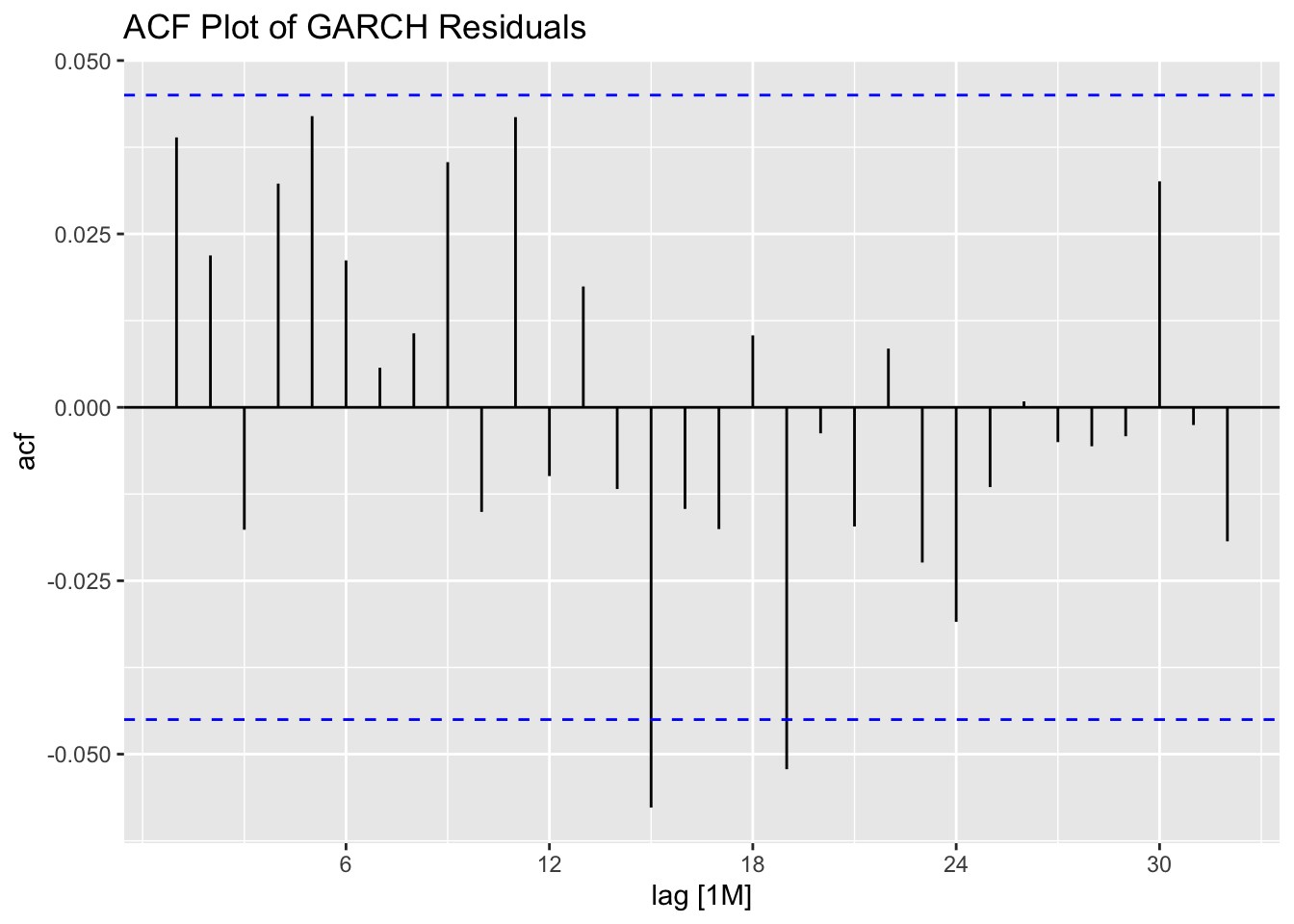

ACF(stemp.garch.res, .resid) |> autoplot() + 
  labs(title = "ACF Plot of GARCH Residuals")

ACF(stemp.garch.res, .resid^2) |> autoplot() + 
  labs(title = "ACF Plot of the Squared GARCH Residuals")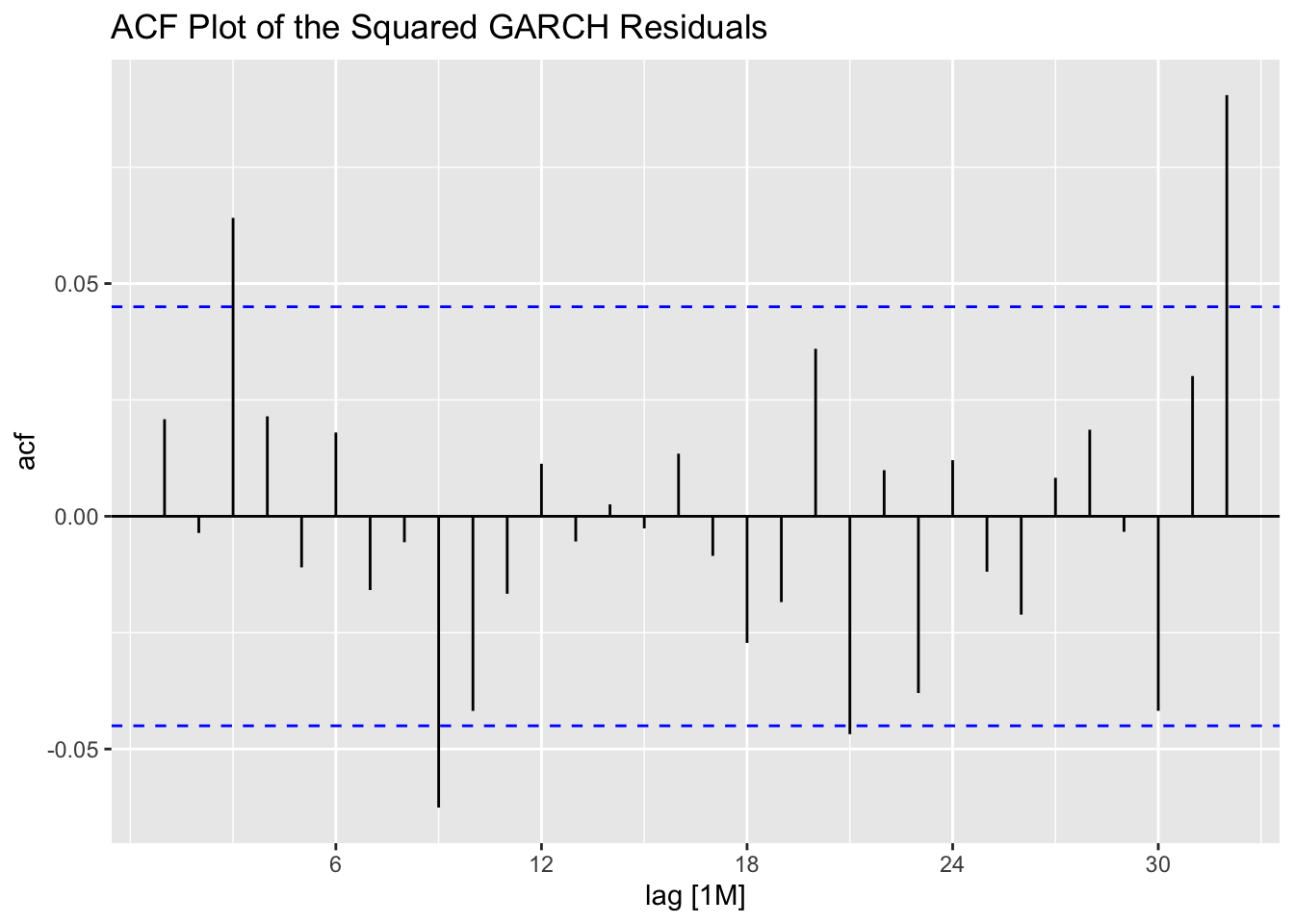

To implement the GARCH model with the ARIMA model above, both the original model and the GARCH model should be used to generate forecasts. The forecasts from each model can then be added together.

6.3 Harmonic Regressions and Fourier Terms

Jean-Baptiste Fourier, a French mathematician showed that a series of \(sin\) and \(cos\) terms with the correct frequencies can approximate any periodic function.⁴³ These terms, dubbed Fourier terms, can be used to approximate seasonal patterns. Included in regressions and ARIMA models, these terms can be a powerful tool in modeling the seasonality present in data.

For example, if \(m\) is the seasonal period, then the first bunch of Fourier terms are:⁴⁴

\[ x_{1,t} = sin(\frac{2 \pi t}{m}), \space x_{2,t} = cos(\frac{2 \pi t}{m}), \space x_{3,t} = sin(\frac{4 \pi t}{m}), \\ x_{4,t} = cos(\frac{4 \pi t}{m}), \space x _{5,t} = sin(\frac{6 \pi t}{m}), x_{6,t} = cos(\frac{6 \pi t}{m}), \text{ ect.} \]

The maximum number of fourier terms allow is \(K = m/2\), where \(m\) is the seasonal period.⁴⁵ The advantages of fourier terms are that they account for any length seasonality and can account for more than one seasonal period through multiple fourier terms.⁴⁶ For more information on fourier terms, refer to this section on harmonic regression

To show examples of different models with fourier components, I will use the aus_retail data from Forecasting: Principles and Practice containing the total monthly expenditure on cafes, restaurants and takeaway food services in Australia ($billion) from 2004 to 2018.⁴⁷

(aus_cafe <- aus_retail |>
  filter(
    Industry == "Cafes, restaurants and takeaway food services",
    year(Month) %in% 2004:2018
  ) |>
  summarise(Turnover = sum(Turnover)) |>
  rename(time = 1))

## # A tsibble: 180 x 2 [1M]
##        time Turnover
##       <mth>    <dbl>
##  1 2004 Jan    1895.
##  2 2004 Feb    1766.
##  3 2004 Mar    1873.
##  4 2004 Apr    1874.
##  5 2004 May    1846 
##  6 2004 Jun    1758.
##  7 2004 Jul    1878.
##  8 2004 Aug    1850.
##  9 2004 Sep    1922.
## 10 2004 Oct    1915.
## # ℹ 170 more rows

The data is monthly, so the seasonal period is 12, meaning K cannot be more than 6. The training set will be the observations from 2004 to 2016 and the test set will be the observations from 2017 to 2018.

First, I examine linear models using all possible fourier terms. I generate measures of accuracy for the training set, forecasts for the training set, and measures of accuracy for the test set. As K increases, generally the amount of error in both the test and training sets both goes down.

aus_cafe.lm <- aus_cafe |>
  filter(year(time) <= 2016) |>
  model(lm = TSLM(log(Turnover) ~ trend()),
        lm1 = TSLM(log(Turnover) ~ trend() + fourier(K = 1)),
        lm2 = TSLM(log(Turnover) ~ trend() + fourier(K = 2)),
        lm3 = TSLM(log(Turnover) ~ trend() + fourier(K = 3)),
        lm4 = TSLM(log(Turnover) ~ trend() + fourier(K = 4)),
        lm5 = TSLM(log(Turnover) ~ trend() + fourier(K = 5)),
        lm6 = TSLM(log(Turnover) ~ trend() + fourier(K = 6)))

accuracy(aus_cafe.lm)

## # A tibble: 7 × 10
##   .model .type       ME  RMSE   MAE     MPE  MAPE  MASE RMSSE   ACF1
##   <chr>  <chr>    <dbl> <dbl> <dbl>   <dbl> <dbl> <dbl> <dbl>  <dbl>
## 1 lm     Training  3.58 140.  102.  -0.138   3.93 0.666 0.780 0.264 
## 2 lm1    Training  2.82 121.   89.5 -0.110   3.51 0.586 0.679 0.0754
## 3 lm2    Training  2.53 115.   90.8 -0.0986  3.54 0.594 0.645 0.0303
## 4 lm3    Training  1.71  93.0  75.9 -0.0676  2.99 0.496 0.520 0.0487
## 5 lm4    Training  1.46  84.2  67.0 -0.0578  2.68 0.438 0.471 0.176 
## 6 lm5    Training  1.00  68.4  54.8 -0.0410  2.22 0.359 0.383 0.718 
## 7 lm6    Training  1.00  68.2  54.5 -0.0409  2.21 0.357 0.381 0.729

aus_cafe.lm.fc <- aus_cafe.lm |> 
  forecast(new_data = aus_cafe |> 
             filter(year(time) > 2016)) 
aus_cafe.lm.fc |>
  accuracy(aus_cafe)

## # A tibble: 7 × 10
##   .model .type    ME  RMSE   MAE   MPE  MAPE  MASE RMSSE    ACF1
##   <chr>  <chr> <dbl> <dbl> <dbl> <dbl> <dbl> <dbl> <dbl>   <dbl>
## 1 lm     Test  -196.  261.  227. -5.47  6.21  1.49  1.46  0.165 
## 2 lm1    Test  -187.  237.  204. -5.14  5.56  1.34  1.33 -0.0778
## 3 lm2    Test  -184.  231.  195. -5.03  5.31  1.28  1.29 -0.140 
## 4 lm3    Test  -181.  210.  181. -4.87  4.88  1.19  1.17 -0.212 
## 5 lm4    Test  -180.  200.  180. -4.83  4.83  1.18  1.12 -0.0470
## 6 lm5    Test  -179.  191.  179. -4.77  4.77  1.17  1.07  0.638 
## 7 lm6    Test  -179.  191.  179. -4.77  4.77  1.17  1.07  0.669

Next, I consider ARIMA models with fourier terms. Additing a fourier term to an ARIMA model creates a linear regression of the dependent variable on the fourier term with ARIMA errors. To make sure ARIMA() does not internally account for the seasonality, PDQ() must be set to 0,0,0. Including both a seasonal ARIMA component and fourier term would not be theoretically consistent, as the seasonality would be accounted for twice.

# THIS TAKES A WHILE TO RUN
aus_cafe.arima <- aus_cafe |>
  filter(year(time) <= 2016) |>
  model(auto = ARIMA(log(Turnover), stepwise = FALSE),
        arima1 = ARIMA(log(Turnover) ~ fourier(K=1) + PDQ(0,0,0)),
        arima2 = ARIMA(log(Turnover) ~ fourier(K=2) + PDQ(0,0,0)),
        arima3 = ARIMA(log(Turnover) ~ fourier(K=3) + PDQ(0,0,0)),
        arima4 = ARIMA(log(Turnover) ~ fourier(K=4) + PDQ(0,0,0)),
        arima5 = ARIMA(log(Turnover) ~ fourier(K=5) + PDQ(0,0,0)),
        arima6 = ARIMA(log(Turnover) ~ fourier(K=6) + PDQ(0,0,0)))

As observed above with the linear models, as K increases the amount of error in the training set decreases. The best fourier model outperforms the ARIMA(3,0,1)(2,1,0)[12] model selected as the best ARIMA model by the algorithm. In the test set, after generating forecasts, the model with the fourier term K = 5 performs the best out of all the models considered.

aus_cafe.arima |> accuracy()

## # A tibble: 7 × 10
##   .model .type       ME  RMSE   MAE      MPE  MAPE  MASE RMSSE     ACF1
##   <chr>  <chr>    <dbl> <dbl> <dbl>    <dbl> <dbl> <dbl> <dbl>    <dbl>
## 1 auto   Training 2.39   52.1  41.0  0.0712   1.60 0.269 0.291 -0.00818
## 2 arima1 Training 3.28  110.   82.1 -0.0518   3.14 0.537 0.614 -0.0442 
## 3 arima2 Training 2.56   85.4  65.5 -0.00317  2.51 0.428 0.477 -0.0444 
## 4 arima3 Training 1.48   69.2  53.1 -0.0110   2.06 0.348 0.387 -0.0446 
## 5 arima4 Training 1.47   58.9  47.5 -0.00158  1.83 0.311 0.329 -0.101  
## 6 arima5 Training 0.702  45.3  36.4 -0.0137   1.44 0.238 0.253 -0.0435 
## 7 arima6 Training 0.717  44.7  35.8 -0.0129   1.42 0.235 0.250 -0.0233

aus_cafe.arima |> select(auto) |> report()

## Series: Turnover 
## Model: ARIMA(3,0,1)(2,1,0)[12] w/ drift 
## Transformation: log(Turnover) 
## 
## Coefficients:
##           ar1     ar2     ar3     ma1     sar1     sar2  constant
##       -0.2266  0.6564  0.3438  0.7738  -0.5799  -0.3753    0.0233
## s.e.   0.2027  0.1506  0.0844  0.2117   0.0879   0.0815    0.0032
## 
## sigma^2 estimated as 0.0004714:  log likelihood=348.02
## AIC=-680.05   AICc=-678.98   BIC=-656.29

aus_cafe.arima.fc <- aus_cafe.arima |> 
  forecast(new_data = aus_cafe |> 
             filter(year(time) > 2016)) 

aus_cafe.arima.fc|>
  accuracy(aus_cafe)

## # A tibble: 7 × 10
##   .model .type     ME  RMSE   MAE   MPE  MAPE  MASE RMSSE    ACF1
##   <chr>  <chr>  <dbl> <dbl> <dbl> <dbl> <dbl> <dbl> <dbl>   <dbl>
## 1 arima1 Test  -224.   264. 235.  -6.12  6.36 1.54  1.48  -0.0403
## 2 arima2 Test  -134.   175. 147.  -3.66  3.98 0.960 0.977 -0.176 
## 3 arima3 Test   -91.6  131. 104.  -2.48  2.79 0.678 0.731 -0.310 
## 4 arima4 Test  -120.   144. 123.  -3.23  3.29 0.802 0.803 -0.281 
## 5 arima5 Test   -96.9  110.  97.1 -2.57  2.58 0.635 0.617  0.538 
## 6 arima6 Test   -99.5  112.  99.5 -2.64  2.64 0.651 0.628  0.575 
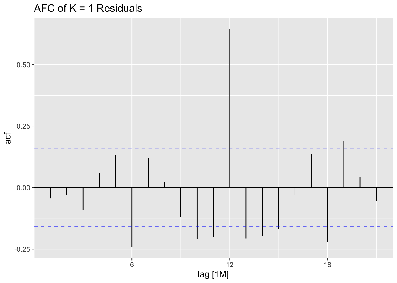
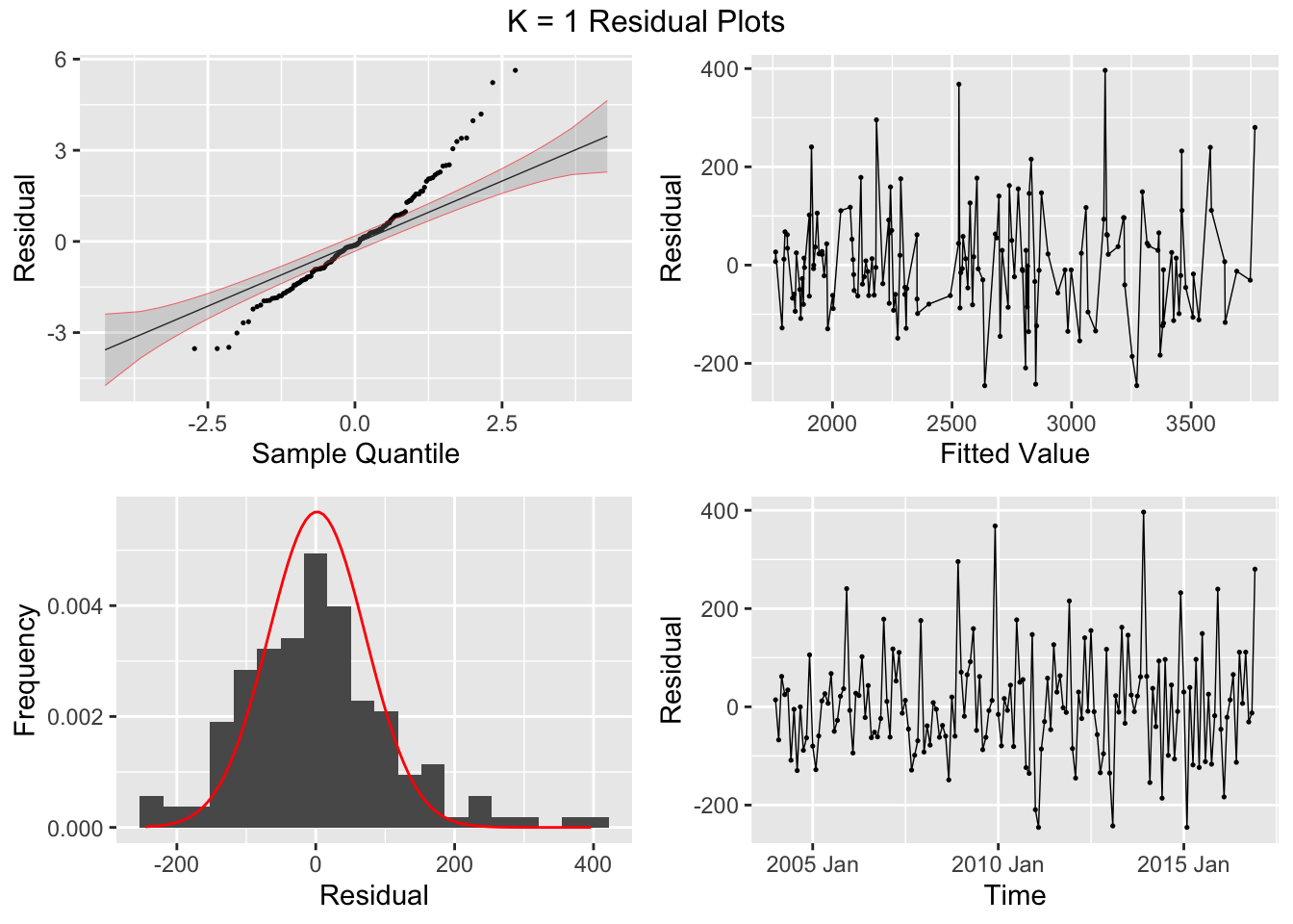
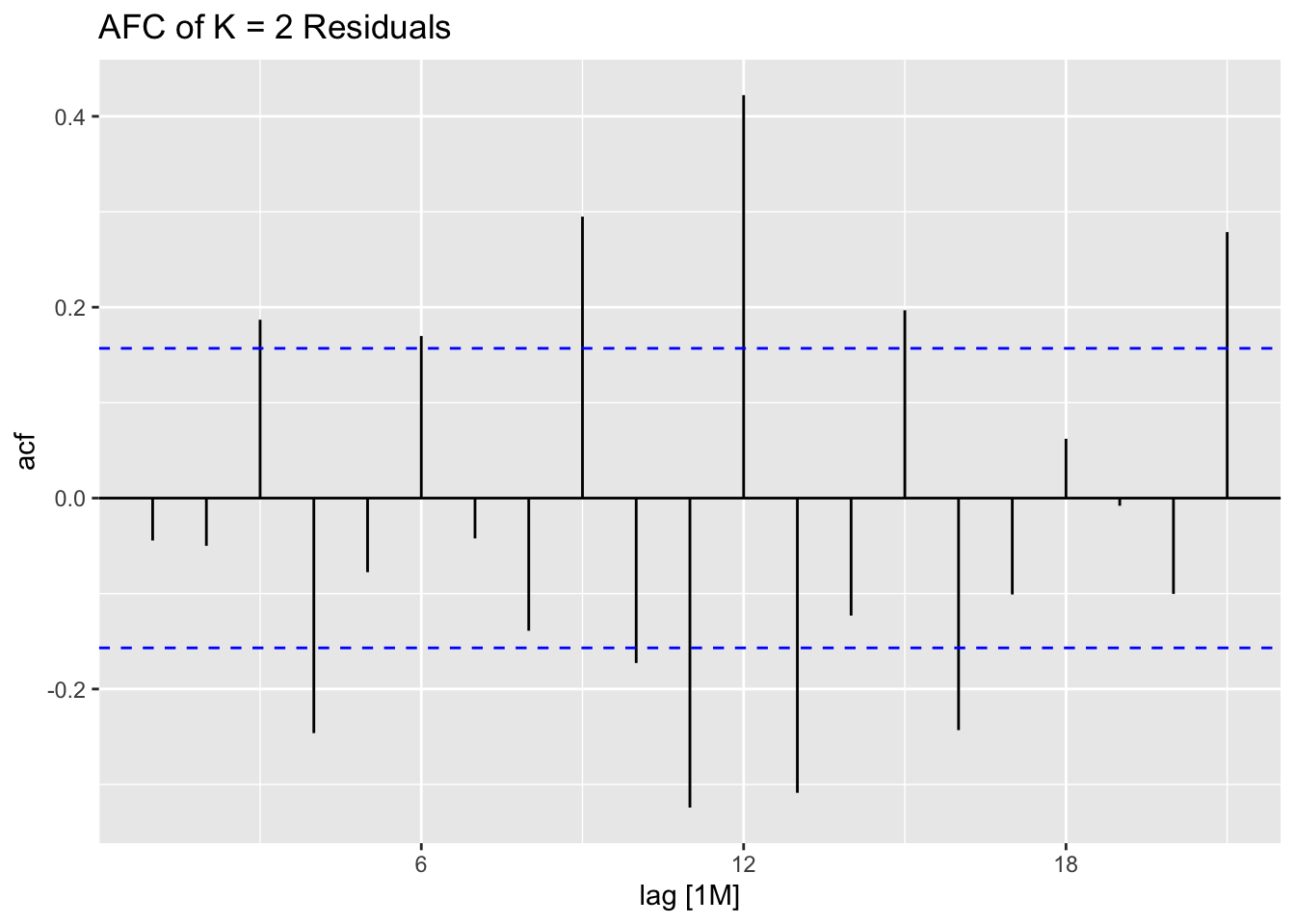
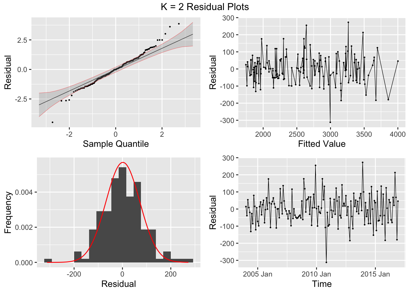
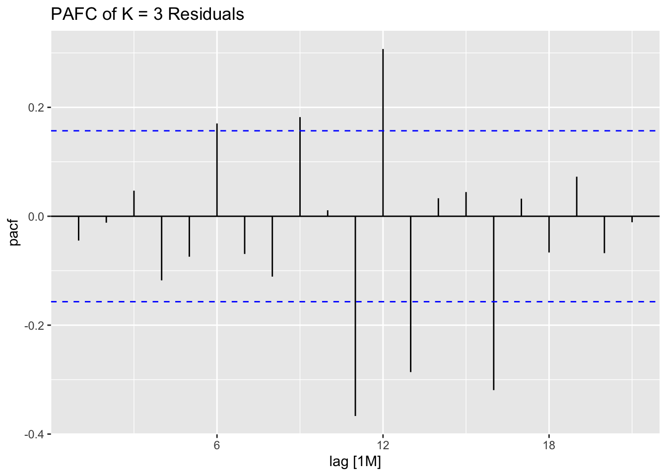
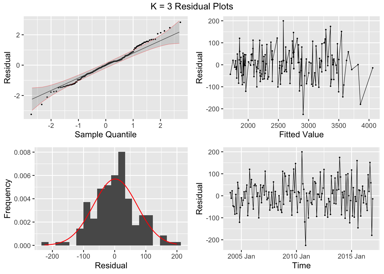
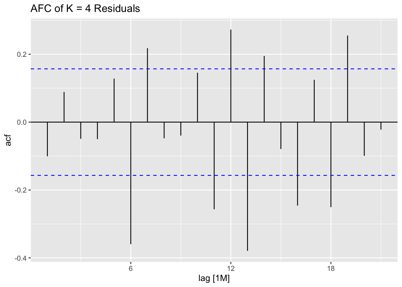
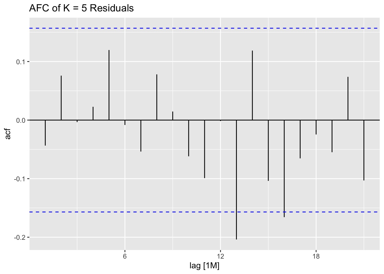
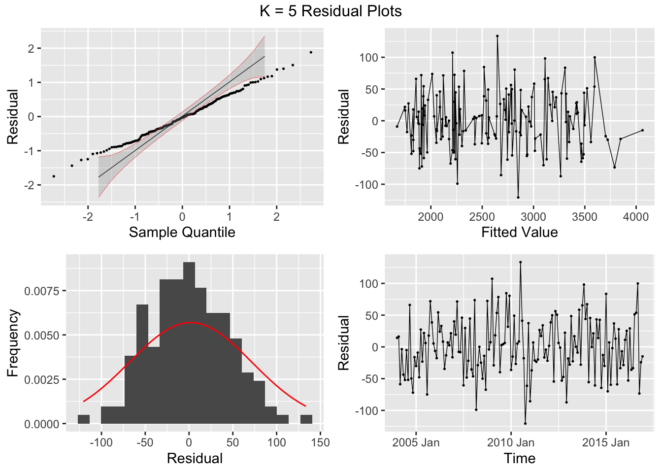
## 7 auto   Test  -123.   135. 123.  -3.26  3.28 0.807 0.756  0.534

augment(aus_cafe.arima) |> plot_residuals(title = c("auto",
                                                    "K = 1",
                                                    "K = 2",
                                                    "K = 3",
                                                    "K = 4",
                                                    "K = 5",
                                                    "K = 6"))

## # A tibble: 7 × 3
##   .model lb_stat lb_pvalue
##   <chr>    <dbl>     <dbl>
## 1 arima1  0.311      0.577
## 2 arima2  0.314      0.576
## 3 arima3  0.317      0.573
## 4 arima4  1.61       0.205
## 5 arima5  0.301      0.583
## 6 arima6  0.0861     0.769
## 7 auto    0.0106     0.918
## # A tibble: 7 × 3
##   .model kpss_stat kpss_pvalue
##   <chr>      <dbl>       <dbl>
## 1 arima1    0.0637         0.1
## 2 arima2    0.0473         0.1
## 3 arima3    0.0564         0.1
## 4 arima4    0.0569         0.1
## 5 arima5    0.0902         0.1
## 6 arima6    0.0895         0.1
## 7 auto      0.0428         0.1

## NULL

References

Hyndman, Rob J, and George Athanasopoulos. Forecasting Principles and Practice. Vol. 3. Melbourne, Australia: OTexts, 2021.

Montgomery, Douglas C, Cheryl L. Jennings, and Murat Kulahci. Introduction to Time Series Analysis and Forecasting. Vol. 2. Hoboken, New Jersey: John Wiley & Sons, 2016.

---

40. Montgomery, Jennings, and Kulahci.↩︎

41. Montgomery, Jennings, and Kulahci.↩︎

42. Montgomery, Jennings, and Kulahci.↩︎

43. Hyndman and Athanasopoulos, Forecasting Principles and Practice.↩︎

44. Hyndman and Athanasopoulos.↩︎

45. Hyndman and Athanasopoulos.↩︎

46. Hyndman and Athanasopoulos.↩︎

47. Hyndman and Athanasopoulos.↩︎