7.3 Hierarchical clustering

Then, we create a new data set that only includes the input variables, i.e., the ratings:

cluster.data <- equipment %>% 
  select(variety_of_choice, electronics, furniture, quality_of_service, low_prices, return_policy) # Select from the equipment dataset only the variables with the standardized ratings

We can now proceed with hierarchical clustering to determine the optimal number of clusters:

# The dist() function creates a dissimilarity matrix of our dataset and should be the first argument to the hclust() function. 
# In the method argument, you can specify the method to use for clustering.
hierarchical.clustering <- hclust(dist(cluster.data), method = "ward.D") 

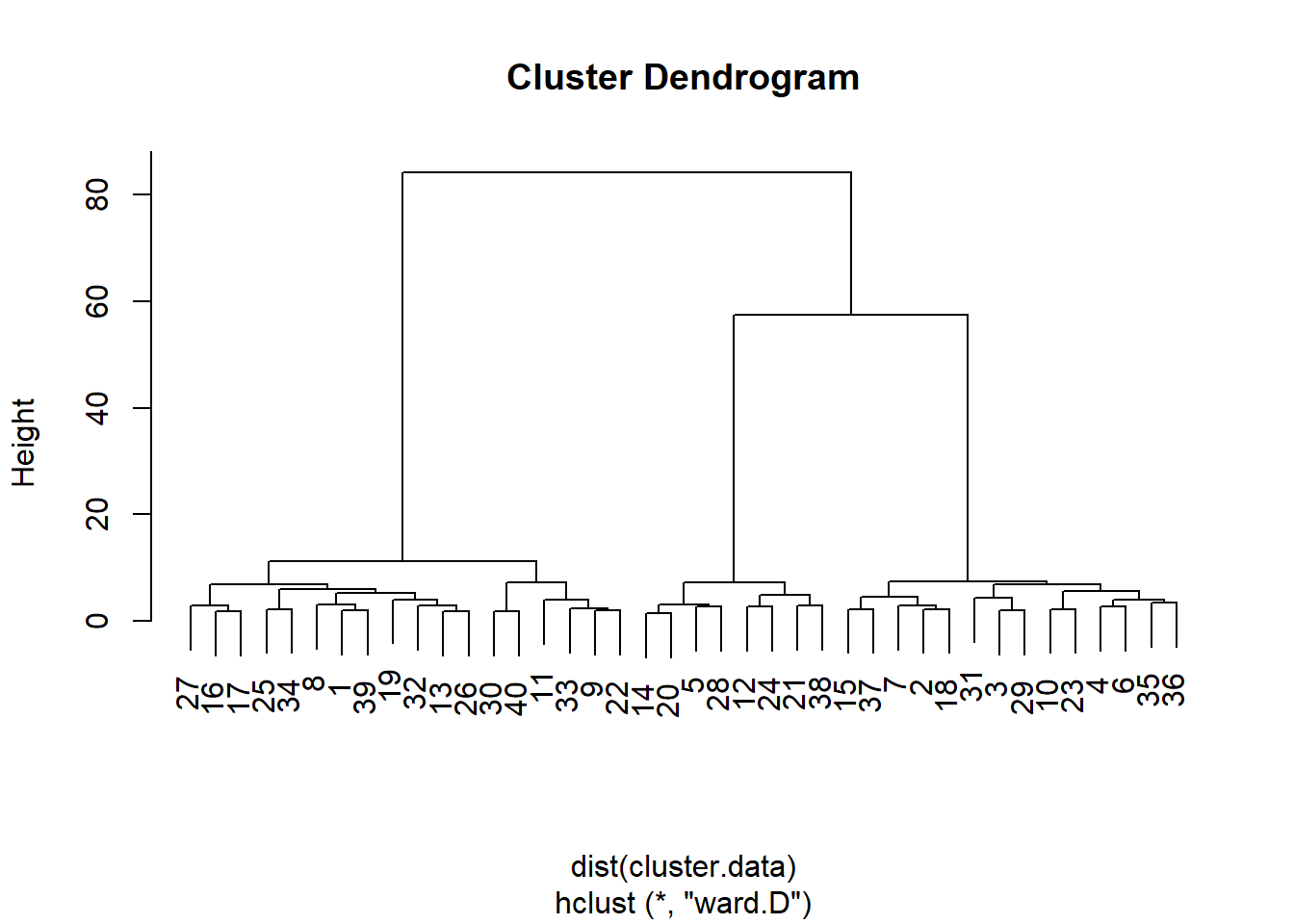
The cluster analysis is stored in the hierarchical.clustering object and can easily be visualized by a dendogram:

plot(hierarchical.clustering)

From this dendogram, it seems that that we can split the observations in either two, three, or six groups of observations. Let’s carry out a formal test, the Duda-Hart stopping rule, to see how many clusters we should retain. For this, we need to (install and) load the NbClust package:

install.packages("NbClust")
library(NbClust)

The Duda-Hart stopping rule table can be obtained as follows:

duda <- NbClust(cluster.data, distance = "euclidean", method = "ward.D2", max.nc = 9, index = "duda")
pseudot2 <- NbClust(cluster.data, distance = "euclidean", method = "ward.D2", max.nc = 9, index = "pseudot2")

duda$All.index

##      2      3      4      5      6      7      8      9 
## 0.2997 0.7389 0.7540 0.5820 0.4229 0.7534 0.5899 0.7036

pseudot2$All.index

##       2       3       4       5       6       7       8       9 
## 46.7352  5.6545  3.9145  4.3091  5.4591  3.2728  3.4757  2.9490

The conventional wisdom for deciding the number of groups based on the Duda-Hart stopping rule is to find one of the largest Duda values that corresponds to a low pseudo-T² value. However, you can also request the optimal number of clusters as suggested by the stopping rule:

duda$Best.nc

## Number_clusters     Value_Index 
##          3.0000          0.7389

In this case, the optimal number is three.