3.3 One-way ANOVA
When your (categorical) independent variable has only two groups, you can test whether the means of the (continuous) dependent variable are significantly different or not with a t-test. When your independent variable has more than two groups, you can test whether the means are different with an ANOVA.
For example, say we want to test whether there is a significant difference between the average prices of entire homes and apartments, private rooms, and shared rooms. Let’s have a look at the means per room type:
airbnb.summary <- airbnb %>%
  group_by(room_type) %>%
  summarize(count = n(), # get the frequencies of the different room types
            mean_price = mean(price), # the average price per room type
            sd_price = sd(price)) # and the standard deviation of price per room type
## `summarise()` ungrouping output (override with `.groups` argument)## # A tibble: 3 x 4
## room_type count mean_price sd_price
## <chr> <int> <dbl> <dbl>
## 1 Entire home/apt 11082 113. 118.
## 2 Private room 6416 64.3 46.5
## 3 Shared room 153 49.6 33.9We can also plot these means in a bar plot:
# When creating a bar plot, the dataset that serves as input to ggplot is the summary with the means, not the full dataset.
# (This is why we have saved the summary above in an object airbnb.summary)

ggplot(data = airbnb.summary, mapping = aes(x = room_type, y = mean_price)) +
  geom_bar(stat = "identity", position = "dodge")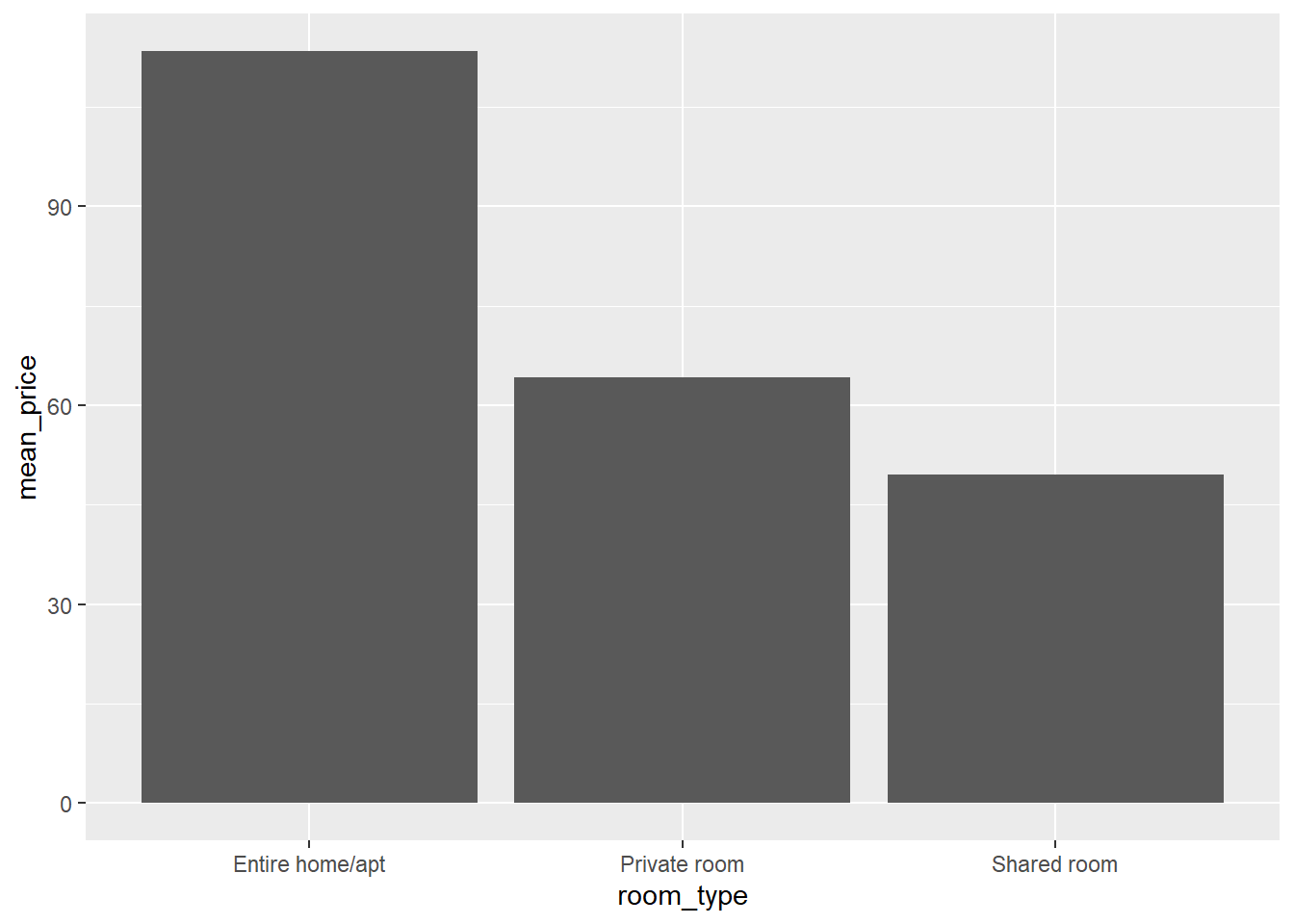
Unsurprisingly, entire homes or apartments are priced higher than private rooms, which in turn are priced higher than shared rooms. We also see that there are almost twice as many entire homes and apartments than private rooms available and there are hardly any shared rooms available. Also, the standard deviation is much higher in the entire homes or apartments category than in the private or shared room categories.
An ANOVA can test whether there are any significant differences in the mean prices per room type. But before we carry out an ANOVA, we need to check whether the assumptions for ANOVA are met.
3.3.1 Assumption: normality of residuals
The first assumption is that the dependent variable (price) is normally distributed at each level of the independent variable (room_type). First, let’s visually inspect whether this assumption will hold:
 # when creating a histogram, the dataset that serves as input to ggplot is the full dataset, not the summary with the means
ggplot(data = airbnb, mapping = aes(x = price)) + # We want price on the X-axis.
  facet_wrap(~ room_type) + # We want this split up per room_type. Facet_wrap will make sure ggplot creates different panels in your graph.
  geom_histogram() # geom_histogram makes sure the frequencies of the values on the X-axis are plotted.
## `stat_bin()` using `bins = 30`. Pick better value with `binwidth`.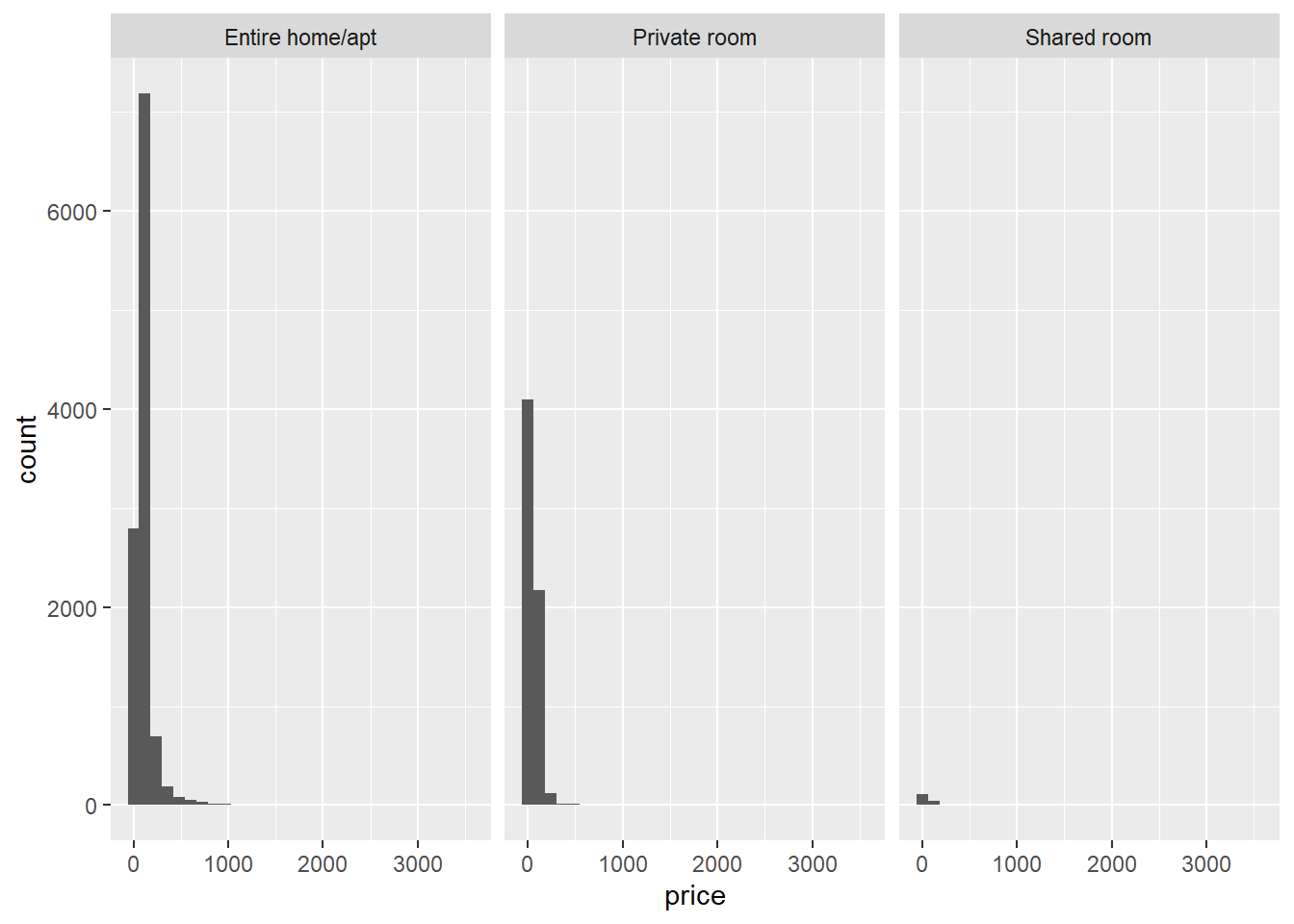
We see that there is right-skew for each room type. We can also formally test, within each room type, whether the distributions are normal with the Shapiro-Wilk test. For example, for the shared rooms:
airbnb.shared <- airbnb %>%
  filter(room_type == "Shared room") # retain data from only the shared rooms

shapiro.test(airbnb.shared$price)
##
## Shapiro-Wilk normality test
##
## data: airbnb.shared$price
## W = 0.83948, p-value = 1.181e-11The p-value of this test is extremely small, so the null hypothesis that the sample comes from a normal distribution should be rejected. If we try the Shapiro-Wilk test for the private rooms:
airbnb.private <- airbnb %>%
  filter(room_type == "Private room") # retain data from only the shared rooms

shapiro.test(airbnb.private$price)
## Error in shapiro.test(airbnb.private$price): sample size must be between 3 and 5000We get an error saying that our sample size is too large. To circumvent this problem, we can try the Anderson-Darling test from the nortest package:
##
##  Anderson-Darling normality test
##
## data:  airbnb.private$price
## A = 372.05, p-value < 2.2e-16
Again, we reject the null hypothesis of normality. I leave it as an exercise to test the normality of the prices of the entire homes and apartments.
Now that we know the normality assumption is violated, what can we do? We can consider transforming our dependent variable with a log-transformation:
ggplot(data = airbnb, mapping = aes(x = log(price, base = exp(1)))) + # We want log-transformed price on the X-axis.
  facet_wrap(~ room_type) + # We want this split up per room_type. Facet_wrap will make sure ggplot creates different panels in your graph.
  geom_histogram() # geom_histogram makes sure the frequencies of the values on the X-axis are plotted.
## `stat_bin()` using `bins = 30`. Pick better value with `binwidth`.![]()
As you can see, a log-transformation normalizes a right-skewed distribution. We could then perform the ANOVA on the log-transformed dependent variable. However, in reality it is often safe to ignore violations of the normality assumption (unless you’re dealing with small samples, which we are not). We’re going to simply carry on with the untransformed price as dependent variable.
3.3.2 Assumption: homogeneity of variances
A second assumption we need to check is whether the variances of our dependent variable price are equal across the categories of our independent variable room_type. Normally, a box plot is informative:
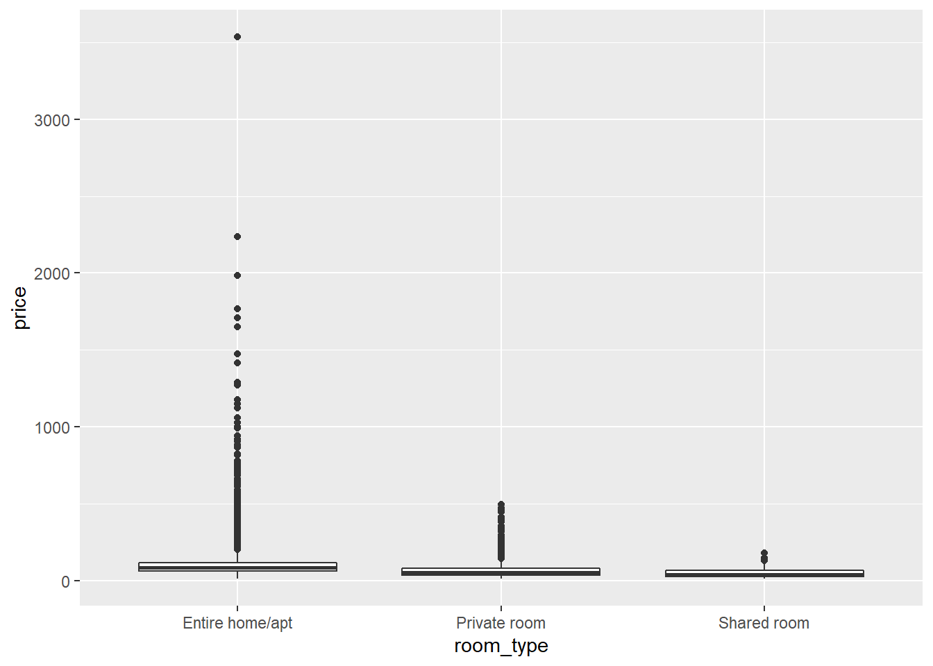
But in this case, the interquartile ranges (the heights of the boxes), which would normally give us an idea of the variance within each room type, are very narrow. This is because the range of Y-values to be plotted is very wide due to some extreme outliers. If we look at the standard deviations, however, we see that these are much higher for the entire rooms and apartments than for the private and shared rooms:
airbnb %>%
  group_by(room_type) %>%
  summarize(count = n(), # get the frequencies of the different room types
            mean_price = mean(price), # the average price per room type
            sd_price = sd(price)) # and the standard deviation of price per room type
## `summarise()` ungrouping output (override with `.groups` argument)## # A tibble: 3 x 4
## room_type count mean_price sd_price
## <chr> <int> <dbl> <dbl>
## 1 Entire home/apt 11082 113. 118.
## 2 Private room 6416 64.3 46.5
## 3 Shared room 153 49.6 33.9We can also carry out a formal test of homogeneity of variances. For this we need the function leveneTest from the package car:
install.packages("car") # For the test of equal variances, we need a package called car. We've installed this before, so no need to re-install it if you have done so already.
library(car)
# Levene's test of equal variances.
# Low p-value means the variances are not equal.
# First argument = continuous dependent variable, second argument = categorical independent variable.
leveneTest(airbnb$price, airbnb$room_type) ## Levene's Test for Homogeneity of Variance (center = median)
## Df F value Pr(>F)
## group 2 140.07 < 2.2e-16 ***
## 17648
## ---
## Signif. codes: 0 '***' 0.001 '**' 0.01 '*' 0.05 '.' 0.1 ' ' 1The p-value is extremely small, so we reject the null hypothesis of equal variances. As with the normality assumption, violations of the assumption of equal variances can, however, often be ignored and we will do so in this case.
3.3.3 The actual ANOVA
To carry out an ANOVA, we need to install some packages:
install.packages("remotes") # The remotes package allows us to install packages that are stored on GitHub, a website for package developers.
install.packages("car") # We'll need the car package as well to carry out the ANOVA (no need to re-install this if you have done this already).

library(remotes)
install_github('samuelfranssens/type3anova') # Install the type3anova package. This and the previous steps need to be carried out only once.

library(type3anova) # Load the type3anova package.
We can now proceed with the actual ANOVA:
# First create a linear model
# The lm() function takes a formula and a data argument
# The formula has the following syntax: dependent variable ~ independent variable(s)
linearmodel <- lm(price ~ room_type, data=airbnb)

# Then ask for output in ANOVA format. This gives Type III sum of squares.
# Note that this is different from anova(linearmodel) which gives Type I sum of squares.
type3anova(linearmodel)
## # A tibble: 3 x 6
## term ss df1 df2 f pvalue
## <chr> <dbl> <dbl> <int> <dbl> <dbl>
## 1 (Intercept) 7618725. 1 17648 803. 0
## 2 room_type 10120155. 2 17648 534. 0
## 3 Residuals 167364763. 17648 17648 NA NAIn this case the p-value associated with the effect of room_type is practically 0, which means that we reject the null hypothesis that the average price is equal for every room_type. You could report this as follows: “There were significant differences between the average prices of different room types (F(2, 17648) = 533.57, p < .001).”
3.3.4 Tukey’s honest significant difference test
Note that ANOVA tests the null hypothesis that the means in all our groups are equal. A rejection of this null hypothesis means that there is a significant difference in at least one of the possible pairs of means (i.e., in entire home/apartment vs. private and/or in entire home/apartment vs. shared and/or in private vs. shared). To get an idea of which pair of means contains a significant difference, we can follow up with Tukey’s test that will give us all pairwise comparisons. Tukey’s test corrects the p-values upwards — so it is more conservative in deciding something is significant — because the comparisons are post-hoc or exploratory:
TukeyHSD(aov(price ~ room_type, data=airbnb),
         "room_type") # The first argument is an "aov" object, the second is our independent variable.
## Tukey multiple comparisons of means
## 95% family-wise confidence level
##
## Fit: aov(formula = price ~ room_type, data = airbnb)
##
## $room_type
## diff lwr upr p adj
## Private room-Entire home/apt -49.11516 -52.69593 -45.534395 0.000000
## Shared room-Entire home/apt -63.79178 -82.37217 -45.211381 0.000000
## Shared room-Private room -14.67661 -33.34879 3.995562 0.155939This shows us that there’s no significant difference in the average price of shared and private rooms, but that shared rooms and private rooms both differ significantly from entire homes and apartments.