2.1 Importing data
In this chapter, we will explore a publicly available dataset of Airbnb data. We found these data here. (These are real data “scraped” from airbnb.com in July 2017. This means that the website owner created a script to automatically collect these data from the airbnb.com website. This is one of the many things that you can also do in R. But first let’s learn the basics.) You can download the dataset by right-clicking on this link, selecting “Save link as…” (or something similar), and saving the .csv file in a directory on your hard drive. As mentioned in the introduction, it’s a good idea to save your work in a directory that is automatically backed up by file-sharing software. Later on, we will save our script in the same directory.
2.1.1 Importing CSV files
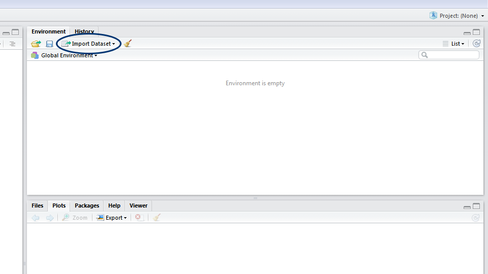
To import data into R, click on Import dataset and then on From text (readr). A new window will pop up. Click on Browse and find your data file. Make sure that First row as names is selected (this tells R to treat the first row of your data as the titles of the columns) and then click on Import. After clicking on import, RStudio opens a Viewer tab. This shows you your data in a spreadsheet.
Some computers save .csv files with semicolons (;) instead of commas (,) as the separators or ‘delimiters’. This usually happens when English is not the first or only language on your computer. If your files are separated by semicolons, click on Import Dataset and find your data file, but now choose Semicolon in the dropdown menu Delimiter.
Note: if you did not save the dataset by right-clicking the link and selecting “Save link as…”, but instead left-clicked the link, then your browser may have ended up opening the dataset. You could then save the dataset by pressing Ctrl+S. Note, however, that your browser may end up saving the dataset as a .txt file. It’s important to then change the extension of your file in the arguments to the read_csv command below.
2.1.2 Setting your working directory
After you have imported your data with Import dataset, check the console window. You’ll see the command for opening the Viewer (View()), and one line above that, you’ll see the command that reads the data. Copy the command that reads the data from the console to your script. In my case it looks like this:
tomslee_airbnb_belgium_1454_2017_07_14 <- read_csv("c:/Dropbox/work/teaching/R/data/tomslee_airbnb_belgium_1454_2017-07-14.csv")
# Change .csv to .txt if necessary.
This line reads as follows (from right to left): the read_csv function should read the tomslee_airbnb_belgium_1454_2017-07-14.csv file from the c:/Dropbox/work/teaching/R/data/ directory (you will see a different directory here). Then, R should assign (<-) these data to an object named tomslee_airbnb_belgium_1454_2017_07_14.
Before we explain each of these concepts, let’s simplify this line of code:
setwd("c:/Dropbox/work/teaching/R/data/") # Set the working directory to where R needs to look for the .csv file
airbnb <- read_csv("tomslee_airbnb_belgium_1454_2017-07-14.csv")
# read_csv now does not require a directory anymore and only needs a filename.
# We assign the data to an object with a simpler name: airbnb instead of tomslee_airbnb_belgium_1454_2017_07_14
The setwd command tells R where your working directory is. Your working directory is a folder on your computer where R will look for data, where plots will be saved, etc. Set your working directory to the folder where you have stored your data. Now, the read_csv file does not require a directory anymore.
You only need to set your working directory once, at the top of your script. You can check whether it’s correctly set by running getwd(). Note that on a Windows computer, file paths have backslashes separating the folders ("C:\folder\data"). However, the filepath you enter into R should use forward slashes ("C:/folder/data").
Save this script in the working directory (in my case: c:/Dropbox/work/teaching/R/data/). In the future you can just run these lines of code to import your data instead of clicking on Import dataset (running lines of code is much faster than pointing and clicking — one of the advantages of using R).
Don’t forget to load the tidyverse package at the top of your script (even before setting the working directory) with library(tidyverse).
2.1.3 Assigning data to objects
Note the <- arrow in the middle of the line that imported the .csv file:
<- is the assignment operator. In this case we assign the dataset (i.e., the data we read from the .csv file) to an object named airbnb. An object is a data structure. All the objects you create will show up in the Environment pane (the top right window). RStudio provides a shortcut for writing <-: Alt + - (in Windows). It’s a good idea to learn this shortcut by heart.
When you import data into R, it will become an object called a data frame. A data frame is like a table or an Excel sheet. It has two dimensions: rows and columns. Usually, the rows represent your observations, the columns represent the different variables. When your data consists of only one dimension (e.g., a sequence of numbers or words), it gets stored in a second type of object called a vector. Later on, we’ll learn how to create vectors.
2.1.4 Importing Excel files
R works best with .csv (comma separated values) files. However, data is often stored as an Excel file (you can download the Airbnb dataset as an Excel file here). R can handle that as well, but you’ll need to load a package called readxl first (this package is part of the tidyverse package, but it does not load with library(tidyverse) because it is not a core tidyverse package):
library(readxl) # load the package

airbnb.excel <- read_excel(path = "tomslee_airbnb_belgium_1454_2017-07-14.xlsx", sheet = "Sheet1")
# make sure the Excel file is saved in your working directory

# you can also leave out path = & sheet =
# then the command becomes: read_excel("tomslee_airbnb_belgium_1454_2017-07-14.xlsx", "Sheet1")
read_excel is a function from the readxl package. It takes two arguments: the first one is the filename and the second argument is the name of the Excel sheet that you want to read.
2.1.5 Inspecting the Airbnb dataset
Our dataset contains information on rooms in Belgium listed on airbnb.com. We know for each room (identified by room_id): who the host is (host_id), what type of room it is (room_type), where it is located (country, city, neighborhood, and even the exact latitude and longitude), how many reviews it has received (reviews), how satisfied people were (overall_satisfaction), price (price), and room characteristics (accommodates, bedrooms, bathrooms, minstay).
A really important step is to check that your data were imported correctly. It’s good practice to always inspect your data — do you see any missing values, do the numbers and names make sense? If you start right away with the analysis, you run the risk of having to re-do your analysis because the data weren’t read correctly, or worse, analysing wrong data without noticing.
## # A tibble: 17,651 x 20
##    room_id survey_id host_id room_type country city  borough neighborhood
##      <dbl>     <dbl>   <dbl> <chr>     <lgl>   <chr> <chr>   <chr>
##  1  5.14e6      1454  2.07e7 Shared r~ NA      Belg~ Gent    Gent
##  2  1.31e7      1454  4.61e7 Shared r~ NA      Belg~ Brussel Schaarbeek
##  3  8.30e6      1454  3.09e7 Shared r~ NA      Belg~ Brussel Elsene
##  4  1.38e7      1454  8.14e7 Shared r~ NA      Belg~ Oosten~ Middelkerke
##  5  1.83e7      1454  1.43e7 Shared r~ NA      Belg~ Brussel Anderlecht
##  6  1.27e7      1454  6.88e7 Shared r~ NA      Belg~ Brussel Koekelberg
##  7  1.55e7      1454  9.91e7 Shared r~ NA      Belg~ Gent    Gent
##  8  3.91e6      1454  3.69e6 Shared r~ NA      Belg~ Brussel Elsene
##  9  1.49e7      1454  3.06e7 Shared r~ NA      Belg~ Vervie~ Baelen
## 10  8.50e6      1454  4.05e7 Shared r~ NA      Belg~ Brussel Etterbeek
## # ... with 17,641 more rows, and 12 more variables: reviews <dbl>,
## #   overall_satisfaction <dbl>, accommodates <dbl>, bedrooms <dbl>,
## #   bathrooms <lgl>, price <dbl>, minstay <lgl>, name <chr>,
## #   last_modified <chr>, latitude <dbl>, longitude <dbl>, location <chr>
R tells us we are dealing with a tibble (this is just another word for data frame) with 17651 rows or observations and 20 columns or variables. For each column, the type of the variable is given: int (integer), chr (character), dbl (double), dttm (date-time). Integer and double variables store numbers (integer for round numbers, double for numbers with decimals), character variables store letters, date-time variables store dates and/or times.
R only prints the data of the first ten rows and the maximum number of columns that fit on the screen. If, however, you want to inspect the whole dataset, double-click on the airbnb object in the Environment pane (the top right window) to open open a Viewer tab or run View(airbnb). Mind the capital V in the View command. R is always case-sensitive!
You can also use the print command to ask for more (or less) rows and columns in the console window:
# Print 25 rows (set to Inf to print all rows) & set width to 100 to see more columns.
# Notice that columns that don't fit on the first screen with 25 rows
# are printed below the initial 25 rows.

print(airbnb, n = 25, width = 100)
## # A tibble: 17,651 x 20
## room_id survey_id host_id room_type country city borough neighborhood
## <dbl> <dbl> <dbl> <chr> <lgl> <chr> <chr> <chr>
## 1 5.14e6 1454 2.07e7 Shared r~ NA Belg~ Gent Gent
## 2 1.31e7 1454 4.61e7 Shared r~ NA Belg~ Brussel Schaarbeek
## 3 8.30e6 1454 3.09e7 Shared r~ NA Belg~ Brussel Elsene
## 4 1.38e7 1454 8.14e7 Shared r~ NA Belg~ Oosten~ Middelkerke
## 5 1.83e7 1454 1.43e7 Shared r~ NA Belg~ Brussel Anderlecht
## 6 1.27e7 1454 6.88e7 Shared r~ NA Belg~ Brussel Koekelberg
## 7 1.55e7 1454 9.91e7 Shared r~ NA Belg~ Gent Gent
## 8 3.91e6 1454 3.69e6 Shared r~ NA Belg~ Brussel Elsene
## 9 1.49e7 1454 3.06e7 Shared r~ NA Belg~ Vervie~ Baelen
## 10 8.50e6 1454 4.05e7 Shared r~ NA Belg~ Brussel Etterbeek
## 11 1.94e7 1454 1.87e7 Shared r~ NA Belg~ Tournai Brunehaut
## 12 1.99e7 1454 1.29e8 Shared r~ NA Belg~ Brussel Etterbeek
## 13 6.77e6 1454 3.50e7 Shared r~ NA Belg~ Gent Gent
## 14 1.39e7 1454 8.18e7 Shared r~ NA Belg~ Arlon Arlon
## 15 1.16e7 1454 5.00e7 Shared r~ NA Belg~ Kortri~ Waregem
## 16 3.65e6 1454 1.84e7 Shared r~ NA Belg~ Antwer~ Boom
## 17 1.20e7 1454 6.37e7 Shared r~ NA Belg~ Vervie~ Büllingen
## 18 1.20e7 1454 6.37e7 Shared r~ NA Belg~ Vervie~ Büllingen
## 19 4.28e5 1454 1.33e6 Shared r~ NA Belg~ Gent Gent
## 20 1.42e7 1454 8.61e7 Shared r~ NA Belg~ Brussel Sint-Jans-M~
## 21 1.93e7 1454 1.07e8 Shared r~ NA Belg~ Leuven Rotselaar
## 22 1.21e7 1454 6.21e7 Shared r~ NA Belg~ Brugge Jabbeke
## 23 4.42e6 1454 2.29e7 Shared r~ NA Belg~ Ath Ath
## 24 1.56e7 1454 2.05e7 Shared r~ NA Belg~ Leuven Leuven
## 25 1.33e6 1454 3.51e6 Shared r~ NA Belg~ Tonger~ Voeren
## reviews overall_satisfa~ accommodates bedrooms bathrooms price minstay name
## <dbl> <dbl> <dbl> <dbl> <lgl> <dbl> <lgl> <chr>
## 1 9 4.5 2 1 NA 59 NA "Spa~
## 2 2 0 2 1 NA 53 NA "app~
## 3 12 4 2 1 NA 46 NA "YOU~
## 4 19 4.5 4 1 NA 56 NA "stu~
## 5 5 5 2 1 NA 47 NA "NIC~
## 6 28 5 4 1 NA 60 NA "Che~
## 7 2 0 2 1 NA 41 NA "a d~
## 8 13 4 2 1 NA 36 NA "Cal~
## 9 2 0 8 1 NA 18 NA "Ecu~
## 10 57 4.5 3 1 NA 38 NA "Bel~
## 11 1 0 4 1 NA 14 NA "Cha~
## 12 0 0 2 1 NA 37 NA "Cos~
## 13 143 5 2 1 NA 28 NA "Cou~
## 14 0 0 1 1 NA 177 NA "Log~
## 15 1 0 4 1 NA 147 NA "Ter~
## 16 3 4.5 2 1 NA 177 NA "PRI~
## 17 0 0 2 1 NA 129 NA "Spa~
## 18 0 0 2 1 NA 140 NA "Spa~
## 19 9 5 2 1 NA 141 NA "pen~
## 20 0 0 5 1 NA 136 NA "App~
## 21 1 0 2 1 NA 132 NA "Hou~
## 22 0 0 1 1 NA 117 NA "Oud~
## 23 0 0 6 1 NA 106 NA "Cha~
## 24 3 5 1 1 NA 116 NA "The~
## 25 13 4.5 2 1 NA 106 NA "Voe~
## # ... with 17,626 more rows, and 4 more variables: last_modified <chr>,
## # latitude <dbl>, longitude <dbl>, location <chr>2.1.6 Importing data from Qualtrics
This section explains how to import data from Qualtrics, which is a popular tool for running online surveys. You can skip this section if you’re working through the Airbnb example.
When you run a survey with Qualtrics, you can download its data by going to ‘Data & Analysis’, pressing ‘Export & Import’ and then ‘Export Data’ (note that a free Qualtrics account will not allow you to download your data, you have to use an institutional account).
Then, you can download your data in different formats.
The format that works best with R is CSV.
You should ‘Download all fields’ and then decide between using numeric values or choice text.
When using numeric values, responses on, e.g., a seven-point Likert scale from 1 = ‘Strongly disagree’ to 7 = ‘Strongly agree’ will be stored as numbers in your .csv file; when using choice text, these responses will be stored as text.
Then you need to download your .csv file.
When you open it, you’ll see a file in which the first three rows are headers.
This complicates a straightforward import into R.
We can resolve this issue as follows:
library(tidyverse)
library(magrittr) # install this first with install.packages("magrittr")

# imagine that your .csv file is named data.csv

variable_names <- read_csv("data.csv") %>% names() # read the dataset and get the variable names from the first row

data <- read_csv("data.csv", skip = 3, col_names = FALSE) %>% # then tell R to read the dataset but skip three rows and not assign variable names
  set_names(variable_names) %>% # we set the variable names that we captured before
  select(-c("IPAddress", "Progress", "RecordedDate", "ResponseId", "RecipientLastName", "RecipientFirstName", "RecipientEmail", "ExternalReference", "DistributionChannel", "UserLanguage")) %>% # remove some variables that you will hardly ever use
  rename(duration = `Duration (in seconds)`) # rename one variable so that there are no spaces in its name

data # Inspect your dataset. This looks much cleaner than the raw dataset that you get from Qualtrics.
If you often use Qualtrics, it makes sense to turn the above into a function that you can often use. Check out the function on my Github page.
Another tip: When you collect data with Qualtrics (or any other survey tool), make sure that you will end up with a data file that has meaningful variable names. Working with variables such as “cognitive_load” and “willingness_to_pay”, instead of “Q1” and “Q2”, is much easier and leads to fewer mistakes. Creating meaningful variable names also makes it much more convenient for others to work with your data. In Qualtrics, you can name your questions and these will become your variable names.