4.3 Two-way ANOVA

When you read an academic paper that reports an experiment, the results section often starts with a discussion of the main effects of the experimental factors and their interaction, as tested by an Analysis of Variance or ANOVA. Let’s focus on WTP for status-enhancing products first. (We have briefly considered the WTP for status-neutral products in our discussion of dependent samples t-tests and we’ll discuss it in more detail in the section on repeated measures ANOVA.)

Let’s inspect some descriptive statistics first. We’d like to view the mean WTP for conspicuous products, the standard deviation of this WTP, and the number of participants in each experimental cell. We’ve already learned how to do some of this in the introductory chapter (see frequency tables and descriptive statistics):

powercc.summary <- powercc %>% # we're assigning the summary to an object, because we'll need this summary to make a bar plot
  group_by(audience, power) %>% # we now group by two variables!
  summarize(count = n(),
            mean = mean(cc),
            sd = sd(cc))

## `summarise()` regrouping output by 'audience' (override with `.groups` argument)

powercc.summary

## # A tibble: 4 x 5
## # Groups:   audience [2]
##   audience power count  mean    sd
##   <fct>    <fct> <int> <dbl> <dbl>
## 1 private  low      34  6.08 1.04 
## 2 private  high     31  5.63 0.893
## 3 public   low      40  6.17 1.15 
## 4 public   high     38  6.07 1.03

We see that the difference in WTP between high and low power participants is larger in the private than in the public condition.

Let’s summarize these results in a box plot:

# when creating a box plot, the dataset that serves as input to ggplot is the full dataset, not the summary with the means
ggplot(data = powercc, mapping = aes(x = audience, y = cc, fill = power)) + 
  geom_boxplot() # arguments are the same as for geom_bar, but now we provide them to geom_boxplot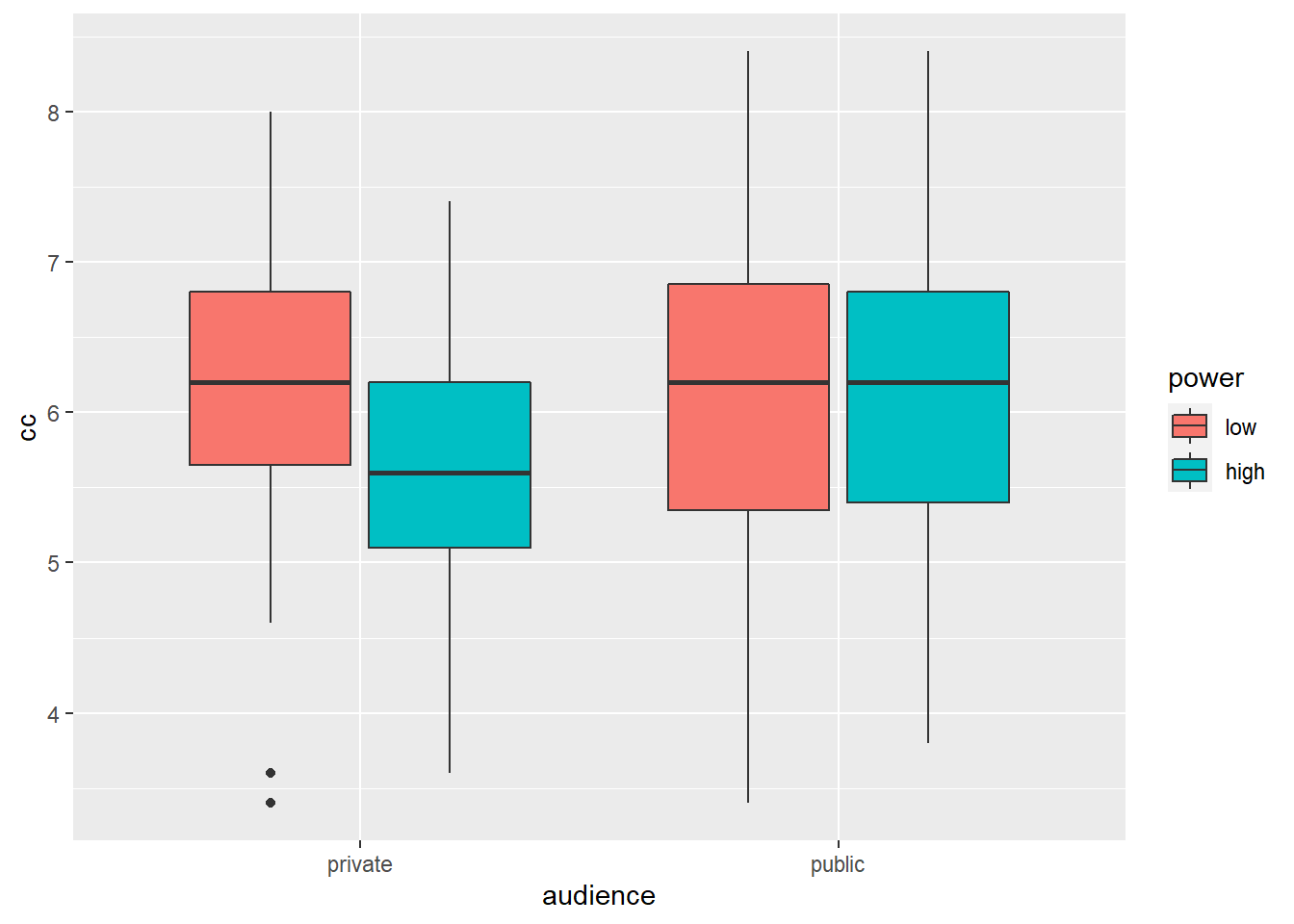

Box plots are informative because they give us an idea of the median and of the distribution of the data. However, in academic papers, the results of experiments are traditionally summarized in bar plots (even though boxplots are more informative).

 # when creating a bar plot, the dataset that serves as input to ggplot is the summary with the means, not the full dataset
ggplot(data = powercc.summary, mapping = aes(x = audience, y = mean, fill = power)) +
  geom_bar(stat = "identity", position = "dodge")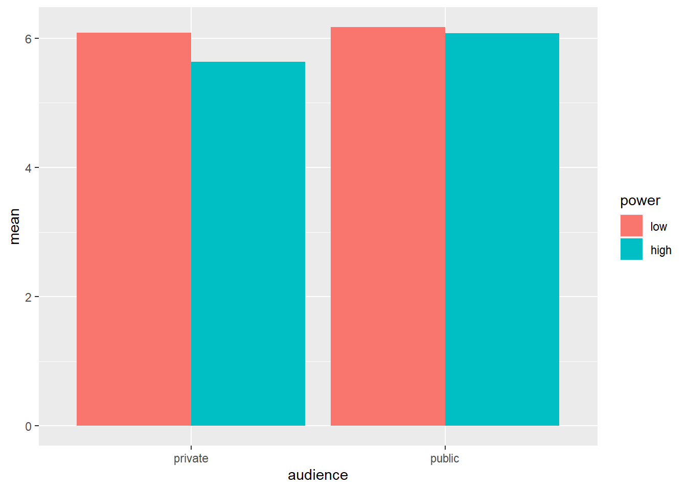

To create a bar plot, we tell ggplot the variables that should be on the X-axis and the Y-axis and we also tell it to use different colors for different levels of power with the fill command. Then we ask for a bar plot with geom_bar. stat = "identity" and position = "dodge" should be included as arguments for geom_bar, but a discussion of these arguments is beyond the scope of this tutorial.

Before we proceed with the ANOVA, we should check whether its assumptions are met. We’ve discussed the assumptions of ANOVA previously, but we skip checking it here.

To carry out an ANOVA, we need to install some packages:

install.packages("remotes") # The remotes package allows us to install packages that are stored on GitHub, a website for package developers. 
install.packages("car") # We'll need the car package as well to carry out the ANOVA (no need to re-install this if you have done this already).

library(remotes)
install_github('samuelfranssens/type3anova') # Install the type3anova package. This and the previous steps need to be carried out only once.

library(type3anova) # Load the type3anova package.

We can now proceed with the actual ANOVA:

# First create a linear model
# The lm() function takes a formula and a data argument
# The formula has the following syntax: dependent variable ~ independent variable(s)
linearmodel <- lm(cc ~ power*audience, data=powercc) 
# power*audience: interaction is included
# power+audience: interaction is not included

type3anova(linearmodel) # Then ask for output in ANOVA format. This gives Type III sum of squares. Note that this is different from anova(linearmodel) which gives Type I sum of squares.

## # A tibble: 5 x 6
##   term                ss   df1   df2       f pvalue
##   <chr>            <dbl> <dbl> <int>   <dbl>  <dbl>
## 1 (Intercept)    5080.       1   139 4710.    0    
## 2 power             2.64     1   139    2.45  0.12 
## 3 audience          2.48     1   139    2.30  0.132
## 4 power:audience    1.11     1   139    1.03  0.313
## 5 Residuals       150.     139   139   NA    NA

You could report these results as follows: “Neither the main effect of power (F(1, 139) = 2.45, p = 0.12), nor the main effect of audience (F(1, 139) = 2.3, p = 0.13), nor the interaction between power and audience (F(1, 139) = 1.03, p = 0.31) was significant.”

4.3.1 Following up with contrasts

When carrying out a 2 x 2 experiment, we’re often hypothesizing an interaction. An interaction means that the effect of one independent variable is different depending on the levels of the other independent variable. In the previous section, the ANOVA told us that the interaction between power and audience was not significant. This means that the effect of high vs. low power was the same in the private and in the public condition and that the effect of public vs. private was the same in the high and in the low power condition. Normally, the analysis would stop with the non-significance of the interaction. However, we’re going to carry out the follow-up tests that one would do if the interaction were significant.

Let’s consider the cell means again:

powercc.summary <- powercc %>% 
  group_by(audience, power) %>% 
  summarize(count = n(),
            mean = mean(cc),
            sd = sd(cc))

## `summarise()` regrouping output by 'audience' (override with `.groups` argument)

# when creating a bar plot, the dataset that serves as input to ggplot is the summary with the means, not the full dataset
ggplot(data = powercc.summary,mapping = aes(x = audience, y = mean, fill = power)) + 
  geom_bar(stat = "identity", position = "dodge")

powercc.summary

## # A tibble: 4 x 5
## # Groups:   audience [2]
##   audience power count  mean    sd
##   <fct>    <fct> <int> <dbl> <dbl>
## 1 private  low      34  6.08 1.04 
## 2 private  high     31  5.63 0.893
## 3 public   low      40  6.17 1.15 
## 4 public   high     38  6.07 1.03

We want to test whether the difference between high and low power within the private condition is significant (low: 6.08 vs. high: 5.63) and whether the difference between high and low power within the public condition is significant (low: 6.17 vs. high: 6.07). To do this, we can use the contrast function from the type3anova library that we’ve installed previously. The contrast function takes two arguments: a linear model and a contrast specification. The linear model is the same as before:

linearmodel <- lm(cc ~ power*audience, data=powercc)

But to know how we should specify our contrast, we need to take a look at the regression coefficients in our linear model:

summary(linearmodel)

## 
## Call:
## lm(formula = cc ~ power * audience, data = powercc)
## 
## Residuals:
##     Min      1Q  Median      3Q     Max 
## -2.7700 -0.6737  0.1177  0.7177  2.3263 
## 
## Coefficients:
##                          Estimate Std. Error t value Pr(>|t|)    
## (Intercept)               6.08235    0.17812  34.148   <2e-16 ***
## powerhigh                -0.45009    0.25792  -1.745   0.0832 .  
## audiencepublic            0.08765    0.24226   0.362   0.7181    
## powerhigh:audiencepublic  0.35378    0.34910   1.013   0.3126    
## ---
## Signif. codes:  0 '***' 0.001 '**' 0.01 '*' 0.05 '.' 0.1 ' ' 1
## 
## Residual standard error: 1.039 on 139 degrees of freedom
## Multiple R-squared:  0.03711,    Adjusted R-squared:  0.01633 
## F-statistic: 1.786 on 3 and 139 DF,  p-value: 0.1527

We have four regression coefficients:

• \(\beta_0\) or the intercept (6.08)
• \(\beta_1\) or the coefficient for “powerhigh”, or the high level of the power factor (-0.45)
• \(\beta_2\) or the coefficient for “audiencepublic”, or the public level of the audience factor (0.09)
• \(\beta_3\) or the coefficient for “powerhigh:audiencepublic” (0.35)

We see that the estimate for the intercept corresponds to the observed mean in the low power, private cell. Add to this the estimate of “powerhigh” and one gets the observed mean in the high power, private cell. Add to the estimate for the intercept, the estimate of “audiencepublic” and one gets the observed mean in the low power, public cell. Add to the estimate for the intercept, the estimate of “powerhigh”, “audiencepublic”, and “powerhigh:audiencepublic” and one gets the observed mean in the high power, public cell. I usually visualize this in a table (and save this in my script) to make it easier to specify the contrast I want to test:

#                   private             public
# low power         b0                  b0+b2
# high power        b0+b1               b0+b1+b2+b3

Say we’re contrasting high vs. low power in the private condition, then we’re testing whether (\(\beta_0\) + \(\beta_1\)) and \(\beta_0\) differ significantly, or whether (\(\beta_0\) + \(\beta_1\)) - \(\beta_0\) = \(\beta_1\) is significantly different from zero. We specify this as follows:

contrast_specification <- c(0, 1, 0, 0) 
# the four numbers correspond to b0, b1, b2, b3. 
# we want to test whether b1 is significant, so we put a 1 in 2nd place (1st place is for b0)

contrast(linearmodel, contrast_specification)

## 
##   Simultaneous Tests for General Linear Hypotheses
## 
## Fit: aov(formula = linearmodel)
## 
## Linear Hypotheses:
##        Estimate Std. Error t value Pr(>|t|)  
## 1 == 0  -0.4501     0.2579  -1.745   0.0832 .
## ---
## Signif. codes:  0 '***' 0.001 '**' 0.01 '*' 0.05 '.' 0.1 ' ' 1
## (Adjusted p values reported -- single-step method)

The output tells us the estimate of the contrast is -0.45, which is indeed the difference between the observed means in the private condition (high power: 5.63 vs. low power: 6.08). You could report this result as follows: “The effect of high (M = 5.63, SD = 0.89) vs. low power (M = 6.08, SD = 1.04) in the private condition was marginally significant (t(139) = -1.745, p = 0.083).” To get the degrees of freedom, do contrast(linearmodel, contrast_specification)$df.

Say we want to test a more complicated contrast, namely whether the mean in the high power, private cell is different from the average of the means in the other cells. We’re testing:

(\(\beta_0\) + \(\beta_1\)) - 1/3 * [(\(\beta_0\)) + (\(\beta_0\) + \(\beta_2\)) + (\(\beta_0\) + \(\beta_1\) + \(\beta_2\) + \(\beta_3\))]

= \(\beta_1\) - 1/3 * (\(\beta_1\) + 2*\(\beta_2\) + \(\beta_3\))

= 2/3 \(\beta_1\) - 2/3 \(\beta_2\) - 1/3 \(\beta_3\)

The contrast specification is as follows:

contrast_specification <- c(0, 2/3, -2/3, -1/3) 
contrast(linearmodel, contrast_specification)

## 
##   Simultaneous Tests for General Linear Hypotheses
## 
## Fit: aov(formula = linearmodel)
## 
## Linear Hypotheses:
##        Estimate Std. Error t value Pr(>|t|)  
## 1 == 0  -0.4764     0.2109  -2.259   0.0254 *
## ---
## Signif. codes:  0 '***' 0.001 '**' 0.01 '*' 0.05 '.' 0.1 ' ' 1
## (Adjusted p values reported -- single-step method)

Check whether the estimate indeed corresponds to the difference between the mean of high power, private and the average of the means in the other cells. You could report this as follows: “The high power, private cell had a significantly lower WTP than the other experimental cells in our design (est = -0.476, t(139) = -2.259, p = 0.025)”.