Chapter 3 Variables Sampling Plans
When actual quantitative information can be measured on sampled items, rather than simply classifying them as conforming or nonconforming, variables sampling plans can be used. To achieve the same operating characteristic, a variables sampling plan requires fewer samples than an attribute plan since more information is available in the measurements. If the measurements do not require much more time and expense than classifying items, the variables sampling plan provides an advantage. When a lot is rejected, the measurements in relation to the specification limits give additional information to the supplier and may help to prevent rejected lots in the future. This is also an advantage of the variables sampling plan.
The disadvantage of variables sampling plans is that they are based on the assumption that the measurements are normally distributed (at least for the plans available in published tables or through pre-written software).
Another critical assumption of variable plans is that the measurement error, in the quantitative information obtained from sampled items, is small relative to the specification limits. If not, the type I and type II errors for the lot acceptance criterion will both be inflated. The standard way of estimating measurement error and comparing it to the specification limits is through the use of a Gauge Repeatability and Reproducibility Study or Gauge R&R study. Section 3.4 will illustrate a basic Gauge R&R study and show R code to analyze the data.
To illustrate the idea of a variables sampling plan, consider the following example. A granulated product is delivered to the customer in lots of 5000 bags. A lower specification limit on the particle size is \(LSL\)=10. A variables sampling plan consists of taking a sample of bags and putting the granulated material in the sampled bags through a series of meshes in order to determine the smallest particle size. This is the measurement. An attribute sampling plan would simply classify each sampled bag containing any particles of size less than the \(LSL\)=10 to be nonconforming or defective, and any bag whose smallest particles are greater than the LSL to be conforming.
There are two different methods for developing the acceptance criteria for a variables sampling plan. The first method is called the k-Method. It compares the standardized difference between the specification limit and the mean of the measurements made on each sampled item to an acceptance constant \(k\). The second method is called the M-Method. It compares the estimated proportion of items out of specifications in the lot to a maximum allowable proportion \(M\). When there is only one specification limit (i.e., \(USL\) or \(LSL\)) the k-method and the M-method yield the same results. When there is both an upper and lower specification limit, the M-method must be used in all but special circumstances.
3.1 The k-Method
3.1.1 Lower Specification Limit
3.1.1.1 Standard Deviation Known
To define a variables sampling plan the number of samples (\(n\)) and an acceptance constant (\(k\)) must be determined. A lot would be accepted if \((\bar{x}-LSL)/\sigma > k\), where \(\bar{x}\) is the sample average of the measurements from a sample and \(\sigma\) is the standard deviation of the measurements. The mean and standard deviation are assumed to be known from past experience. In terms of the statistical theory of hypothesis testing, accepting the lot would be equivalent to failing to reject the null hypothesis \(H_0: \mu \ge \mu_{AQL}\) in favor of the alternative \(H_a: \mu<\mu_{AQL}\).
When the measurements are assumed to be normally distributed with a lower specification limit \(LSL\), the AQL and the RQL in terms of proportion of items below the \(LSL\) can be visualized as areas under the normal curve to the left of the LSL as shown in Figure 3.1. In this figure it can be seen that when the mean is \(\mu_{AQL}\) the proportion of defective items is AQL, and when the mean of the distribution is \(\mu_{RQL}\) the proportion of defective items is RQL.
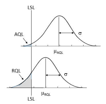
Figure 3.1 AQL and RQL for Variable Plan
If the producer’s risk is \(\alpha\) and the consumer’s risk is \(\beta\), then \[\begin{equation} P \left( \frac{\bar{x}-LSL}{\sigma}>k \mid\mu=\mu_{AQL} \right) = 1-\alpha \tag{3.1} \end{equation}\] and \[\begin{equation} P \left( \frac{\bar{x}-LSL}{\sigma}>k \mid\mu=\mu_{RQL} \right) = \beta. \tag{3.2} \end{equation}\]
In terms statistical hypothesis testing, Equation (3.1) is equivalent to having a significance level of \(\alpha\) for testing \(H_0: \mu \ge \mu_{AQL}\), and Equation (3.2) is equivalent to having power of \(1-\beta\) when \(\mu=\mu_{RQL}\).
By multiplying both sides of the inequality inside the parenthesis in Equation (3.1) by \(\sqrt{n}\), subtracting \(\frac{\mu_{AQL}}{\sigma/\sqrt{n}}\) from each side, and adding \(\frac{LSL}{\sigma/\sqrt{n}}\) to each side, it can be seen that
\[\begin{equation} \frac{\bar{x}-LSL}{\sigma}>k \Rightarrow \frac{\bar{x}-\mu_{AQL}}{\sigma/\sqrt{n}}>k\sqrt{n}+\frac{LSL-\mu_{AQL}}{\sigma/\sqrt{n}}. \tag{3.3} \end{equation}\]
If the mean is given as \(\mu=\mu_{AQL}\), then \(\frac{\bar{x}-\mu_{AQL}}{\sigma/\sqrt{n}}\) follows the standard normal distribution with mean \(\mu=0\) and standard deviation \(\sigma=1\). Therefore, \[\begin{equation} \begin{split} P\left(Z>k\sqrt{n}+\frac{LSL-\mu_{AQL}}{\sigma/\sqrt{n}}\right)&=1-\alpha,\\ \\ \textrm{and}\\ \\ P\left(Z<k\sqrt{n}+\frac{LSL-\mu_{AQL}}{\sigma/\sqrt{n}}\right)&=\alpha.\\ \end{split} \tag{3.4} \end{equation}\]
Consequently, \[\begin{equation} \begin{split} k\sqrt{n}+&\frac{LSL-\mu_{AQL}}{\sigma/\sqrt{n}}=Z_{\alpha}\\ \\ &\textrm{or}\\ \\ k=\frac{Z_{\alpha}}{\sqrt{n}}-&\frac{LSL-\mu_{AQL}}{\sigma}=\frac{Z_{\alpha}}{\sqrt{n}}-Z_{AQL},\\ \\ \textrm{since} \;\;&\frac{LSL-\mu_{AQL}}{\sigma}= Z_{AQL}. \end{split} \tag{3.5} \end{equation}\]
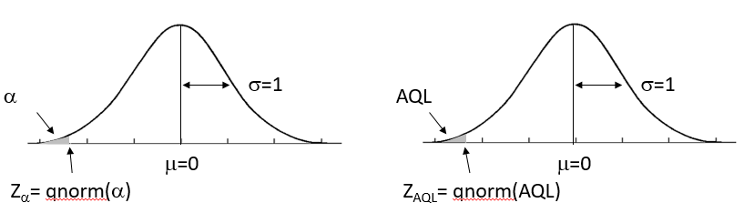
Figure 3.2 Standard Normal Quantile \(Z_{\alpha}\) and \(Z_{AQL}\)
Performing the same manipulations with the inequality in Equation (3.2), it can be shown that \[\begin{equation} k=\frac{Z_{1-\beta}}{\sqrt{n}}-Z_{RQL}. \tag{3.6} \end{equation}\]
Equating the solution for \(k\) in the next to last line in Equation (3.5) with the solution for \(k\) in Equation (3.6) and solving for \(n\), it can be seen that \[\begin{equation} \frac{Z_{\alpha}}{\sqrt{n}}-Z_{AQL}=\frac{Z_{1-\beta}}{\sqrt{n}}-Z_{RQL}\Rightarrow n=\left(\frac{Z_{\alpha}-Z_{1-\beta}}{Z_{AQL}-Z_{RQL}}\right)^2. \tag{3.7} \end{equation}\]
\(Z_{\alpha}\), \(Z_{AQL}\), and \(Z_{RQL}\) are quantiles of the standard normal distribution, as shown in Figure (3.2). They can be calculated with the R function \(\verb!qnorm!\). For the case where AQL=1% or 0.01, the RQL=4.6% or 0.046, \(\alpha=0.05\) and \(\beta=0.10\), the R Code below evaluates Equation (3.7) and the last line of Equation (3.5) to find the sample size \(n\) and the acceptance constant \(k\) for a custom variable sampling plan that has PRP=(.01,.95), and CRP=(.046,.10).
The first line of code calculates \(n=\) 20.8162. This is rounded up to the next integer (21) which is substituted into the next line for for \(n\) in calculating \(k=\) 1.967411.
Thus, conducting the sampling plan on a lot of material consists of the following steps:
- Take a random sample of \(n\) items from the lot
- Measure the critical characteristic \(x\) on each sampled item
- Calculate the mean measurement \(\overline{x}\)
- Compare \((\overline{x}-LSL)/\sigma\) to the acceptance constant \(k=\) 1.967411
- If \((\overline{x}-LSL)/\sigma >k\), accept the lot, otherwise reject the lot.
The R code below uses the \(\verb!OCvar()!\) function in the \(\verb!AcceptanceSampling!\) package to store the plan and make the OC curve shown in Figure 3.3.
library(AcceptanceSampling)
plnVkm<-OCvar(21,1.967411,pd=seq(0,.15,.001))
plot(plnVkm, type='l')
grid()
Figure 3.3 OC Curve for Variables Sampling Plan \(n = 21\), \(k = 1.967411\)
This OC curve is very steep and close to the ideal with a very high probability of accepting lots with 1% defective or less, and a very low probability of accepting lots with 4.6% defective or more.
The \(\verb!find.plan()!\) function in the \(\verb!AcceptanceSampling!\) package automates the procedure of finding the sample size (\(n\)) and acceptance constant (\(k\)) for a custom derived variables sampling plan. The R code and output below shows how this is done.
library(AcceptanceSampling)
find.plan(PRP=c(0.01, 0.95), CRP=c(0.046, 0.10), type="normal")
$n
[1] 21

$k
[1] 1.967411

$s.type
[1] "known"
If the items in the sample could only be classified as nonconforming or conforming, an attribute sampling plan would require many more samples to have a equivalent OC curve. The R code and output below uses the \(\verb!find.plan()!\) function in the \(\verb!AcceptanceSampling!\) package to find an equivalent custom derived attribute sampling plan and plot the OC curve shown in Figure 3.4. The \(\verb!type="binomial"!\) option in the \(\verb!find.plan()!\) was used assuming that the lot size is large enough that the Binomial distribution is an accurate approximation to the Hypergeometric distribution for calculating the probability of acceptance with the attribute plan.
library(AcceptanceSampling)
find.plan(PRP=c(0.01, 0.95), CRP=c(0.046, 0.10), type="binomial")
$n
[1] 172

$c
[1] 4

$r
[1] 5

plnA<-OC2c(n=172,c=4, type="binomial",pd=seq(0,.15,.001))
plot(plnA,type='l', xlim=c(0,.15))
grid()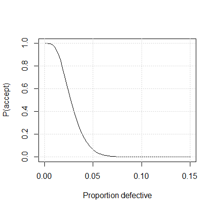
Figure 3.4 OC Curve for Attribute Sampling Plan \(n = 172\), \(c = 4\)
We can see that the OC curve for the attribute sampling plan in Figure 3.4 is about the same as the OC curve for the variables sampling plan in Figure 3.3, but the sample size \(n=\) 172 required for the attribute plan is much higher than the sample size \(n=\) 21 for the variable plan. The variable plan would be advantageous unless the effort and expense of making the measurements took more than 8 times the effort and expense of simply classifying the items as conforming to specifications or not.
Example 1 (Mitra 1998) presents the following example of the use of a variables sampling plan with a lower specification limit and the standard deviation known. In the the manufacture of heavy-duty utility bags for household use, the lower specification limit on the carrying weight is 100 kg. The AQL is 0.02 or 2%, the RQL is 0.12 or 12%. The producers risk \(\alpha =\) 0.08, and the consumers risk \(\beta =\) 0.10, and the standard deviation of the carrying weight is \(\sigma =\) 8 kg. The R Code and output below shows the sample size \(n =\) 10, and the acceptance constant \(k =\) 1.6009 for the custom derived sampling plan.
library(AcceptanceSampling)
find.plan(PRP=c(.02,.92), CRP=c(.12,.10), type='normal')
$n
[1] 10

$k
[1] 1.609426

$s.type
[1] "known"
After selecting a sample of \(n =\) 10 bags, the average carrying weight was found to be \(\overline{x} = 110\). Then, \[\begin{equation*} Z_L=\frac{\overline{x}-LSL}{\sigma}=\frac{110-100}{8}= 1.25 < 1.609 = k \end{equation*}\]
Therefore, reject the lot.
3.1.1.2 Standard Deviation Unknown
If it could not be assumed that the standard deviation \(\sigma\) were known, the \(Z_{\alpha}\) and \(Z_{1-\beta}\) in Equation 3.7 would have to be replaced with the quantiles of the \(t\)-distribution with \(n-1\) degrees of freedom (\(t_{\alpha}\) and \(t_{1-\beta}\) ). Then Equation 3.7 could not directly be solved for \(n\), because the right side of the equation is also a function \(n\). Instead an iterative approach would have to be used to solve for \(n\). The \(\verb!find.plan()!\) function in the \(\verb!AcceptanceSampling!\) package does this as illustrated below.
library(AcceptanceSampling)
find.plan(PRP=c(0.01, 0.95), CRP=c(0.046, 0.10), type="normal", s.type="unknown")
$n
[1] 63

$k
[1] 1.974026

$s.type
[1] "unknown"
The sample size \(n=63\) for this plan with \(\sigma\) unknown is still much less than the n=172 that would be required for the attribute sampling plan with an equivalent OC curve.
The R code below uses the \(\verb!OC2c()!\), and \(\verb!OCvar()!\) functions in the \(\verb!AcceptanceSampling!\) package to store the plans for the attribute sampling plan (whose OC curve is shown in Figure 3.4) and the variable sampling plans for the cases where \(\sigma\) is unknown or known. The values operating characteristic OC can be retrieved from each plan by attaching the suffix \(\verb!@paccept!\) to the names for the stored plans. The OC curves for each plan are then plotted on the same graphin Figure 3.5 using the R \(\verb!plot!\) function for comparison.
library(AcceptanceSampling)
PD<-seq(0,.15,.001)
plnA<-OC2c(n=172,c=4,type="binomial",pd=PD)
plnVku<-OCvar(n=63,k=1.974026,pd=PD,s.type="unknown")
plnVkm<-OCvar(n=21,k=1.96411,pd=PD,s.type="known")
#Plot all three OC curves on the same graph
plot(PD,plnA@paccept,type='l',lty=1,col=1,xlab='Probability of nonconforming',ylab='OC')
lines(PD,plnVku@paccept,type='l',lty=2,col=2)
lines(PD,plnVkm@paccept,type='l',lty=4,col=4)
legend(.04,.95,c("Attribute","Variable, sigma unknown","Variable, sigma known"),lty=c(1,2,4),
       col=c(1,2,4))
grid()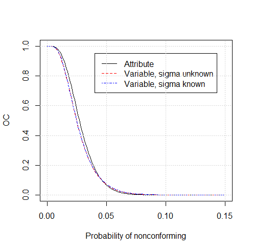
Figure 3.5 Comparison of OC Curves for Attribute and Variable Sampling Plans
It can be seen in Figure 3.5 that the OC curve for the two variable plans are essentially identical, although the sample size (\(n\)=21) is less when \(\sigma\) is known. The OC curves for these variable plans are very similar to the OC curve for the attribute plan (that is also shown in Figure 3.4), but they do offer the customer slightly more protection for intermediate values of the proportion nonconforming, as can be seen in Figure 3.5.
When the standard deviation is unknown, conducting the sampling plan on a lot of material consists of the following steps:
- Take a random sample of \(n\) items from the lot
- Measure the critical characteristic \(x\) on each sampled item
- Calculate the mean measurement \(\overline{x}\), and the sample standard deviation \(s\)
- Compare \((\overline{x}-LSL)/s\) to the acceptance constant \(k\)
- If \((\overline{x}-LSL)/s >k\), accept the lot, otherwise reject the lot.
Example 2 (Montgomery 2013) presents the following example of the use of a custom derived variables sampling plan with a lower specification limit and standard deviation unknown. A soft drink bottler buys nonreturnable bottles from a supplier. Their lower specification limit on the bursting strength is 225psi. The AQL is 0.01 or 1%, the RQL is 0.06 or 6%. The producers risk \(\alpha =\) 0.05, and the consumers risk \(\beta =\) 0.10, and the standard deviation of the bursting strength is unknown. The R Code and output below show the sample size \(n =\) 42, and the acceptance constant \(k =\) 1.905285.
library(AcceptanceSampling)
find.plan(PRP=c(.01,.95), CRP=c(.06,.10), type='normal',s.type='unknown')
$n
[1] 42

$k
[1] 1.905285

$s.type
[1] "unknown"
After selecting a sample of \(n =\) 42 bottles, the average bursting strength was found to be \(\overline{x} = 255\), with a sample standard deviation of \(s =\) 15. Then, \[\begin{equation*} Z_L=\frac{\overline{x}-LSL}{s}=\frac{255-225}{15}= 2.0 > 1.905285 = k \end{equation*}\]
Therefore, accept the lot.
3.1.2 Upper Specification Limit
3.1.2.1 Standard Deviation Known
If a variables sampling plan was required for a situation where there was an upper specification limit (USL), instead of a lower specification limit (LSL), then the fourth and fifth steps in conducting the sampling plan on a lot of material would change from:
- Compare \((\overline{x}-LSL)/\sigma\) to the acceptance constant \(k\)
- If \((\overline{x}-LSL)/\sigma >k\), accept the lot, otherwise reject the lot.
to
- Compare \((USL-\overline{x})/\sigma\) to the acceptance constant \(k\)
- If \((USL-\overline{x})/\sigma >k\), accept the lot, otherwise reject the lot.
3.1.2.2 Standard Deviation Unknown
If the standard deviation were unknown, steps 4 and 5 above would change to
- Compare \((USL-\overline{x})/s\) to the acceptance constant \(k\)
- If \((USL-\overline{x})/s >k\), accept the lot, otherwise reject the lot.
and the sample size \(n\) and acceptance constant \(k\) would be found with the \(\verb!find.plan()!\) function, as shown in the example code below.
3.1.3 Upper and Lower Specification Limits
3.1.3.1 Standard Deviation Known.
When there is an upper (USL) and a lower specification limit (LSL), (Schilling and Neubauer 2017) proposed a simple procedure that may be used to determine if two separate single specification limit plans may be used. The procedure is as follows:
- Calculate \(Z_{p*} = (LSL-USL)/2\sigma\)
- Calculate \(p*\) = \(\verb!pnorm!(Z_{p*}\)) the area under the standard normal density to the left of \(Z_{p*}\).
- If \(2p* \ge RQL\) reject the lot, because even if the distribution is centered between the specification limits, the a proportion outside the specification limits will be too high.
- If \(2p* \le AQL\) use two single specification sampling plans (i.e., one for LSL and one for USL).
- If \(AQL \le 2p* \le RQL\) then use the M-Method for upper and lower specification limits that is described in Section 3.2
3.1.3.2 Standard Deviation Unknown
When there is an upper (USL) and a lower specification limit (LSL), and the standard deviation is unknown, use the M-Method described in Section 3.2.
3.2 The M-Method
3.2.1 Lower Specification Limit
3.2.1.1 Standard Deviation Known
For a variables sampling plan, the M-Method compares the estimated proportion below the \(LSL\) to a maximum allowable proportion. In this case, the uniform minimum variance unbiased estimate of the proportion below the \(LSL\) developed by (Lieberman and Resnikoff 1955) is used. The maximum allowable proportion below \(LSL\) is a function of the acceptance constant \(k\) used in the k-method. For the case of a lower specification limit and the standard deviation known, the uniform minimum variance unbiased estimate of the proportion defective is: \[\begin{equation} P_L=\int_{Q_L}^{\infty} \frac{1}{\sqrt{2\pi}} e^{-t^2/2} dt, \tag{3.8} \end{equation}\] or the area under the standard normal distribution to the right of \(Q_L=Z_L\left(\sqrt{\frac{n}{n-1}}\right)\),
where \(Z_L=(\overline{x}-LSL)/\sigma\). The maximum allowable proportion defective is:
\[\begin{equation} M=\int_{k\sqrt{\frac{n}{n-1}}}^{\infty} \frac{1}{\sqrt{2\pi}} e^{-t^2/2} dt, \tag{3.9} \end{equation}\] or the area under the standard normal distribution to the right of \(k\sqrt{\frac{n}{n-1}}\), where \(k\) is the acceptance constant used in the k-method.
Example 3 To illustrate, reconsider Example 1 from [Mitra (1998)}. The sample size was \(n =\) 10, and the acceptance constant was \(k =\) 1.6094. The lower specification limit was \(LSL =\) 100, and the known standard deviation was \(\sigma =\) 8. In the sample of 10, \(\overline{x} =\) 110. Therefore, \(Q_L=\left(\frac{110-100}{8}\right)\left(\sqrt{\frac{10}{9}}\right)=1.3176\). The estimated proportion defective and the R command to evaluate it is: \[\begin{equation*} P_L=\int_{1.3176}^{\infty} \frac{1}{\sqrt{2\pi}} e^{-t^2/2} dt= \verb!1-pnorm(1.3176)!=0.0938. \end{equation*}\]
The maximum allowable proportion defective and the R command to evaluate it is: \[\begin{equation*} M=\int_{1.6094\sqrt{\frac{10}{9}}}^{\infty} \frac{1}{\sqrt{2\pi}} e^{-t^2/2} dt = \verb!1-pnorm(1.6094*sqrt(10/9))!=0.0449. \end{equation*}\]
Since 0.0938 > 0.0449 (or \(P_L > M\)), reject the lot. This is the same conclusion reached with the k-method shown in Example 1. When there is only one specification limit the results of the k-method and the M-method will always agree.
\(M\) and \(P_L\) can be calculated with the R function \(\verb!pnorm!\) or alternatively with the \(\verb!MPn()!\) and \(\verb!EPn()!\) functions in the R package \(\verb!AQLSchemes!\) as shown in the code below.
3.2.1.2 Standard Deviation Unknown
When the standard deviation is unknown, the symmetric standardized Beta distribution is used instead of the standard normal distribution in calculating the uniform minimum variance unbiased estimate of the proportion defective. The standardized Beta CDF is defined as
\[\begin{equation}
B_x(a,b)=\frac{\Gamma(a+b)}{\Gamma(a)\Gamma(b)}\int_0^x\nu^{a-1}(1-\nu)^{b-1} d\nu,
\tag{3.10}
\end{equation}\]
where \(0\le x \le 1\), \(a>0\), and \(b>0\). The density function is symmetric when \(a = b\).
The estimate of the proportion defective is then
\[\begin{equation}
\hat{p}_L=B_x(a,b),
\tag{3.11}
\end{equation}\]
where \(a=b=\frac{n}{2}-1\), and
\[\begin{equation*}
x=\max \left( 0, .5-.5Z_L\left(\frac{\sqrt{n}}{n-1}\right) \right),
\end{equation*}\]
and the sample standard deviation \(s\) is substituted for \(\sigma\) in the formula for
\[\begin{equation*}
Z_L=\frac{\overline{x}-LSL}{s}.
\end{equation*}\]
When the standard deviation is unknown, the maximum allowable proportion defective is calculated as:
\[\begin{equation} M=B_{B_M}\left(\frac{n-2}{2},\frac{n-2}{2}\right), \tag{3.12} \end{equation}\]
where \[\begin{equation*} B_M=.5\left(1-k\frac{\sqrt{n}}{n-1} \right), \end{equation*}\] and \(k\) is the acceptance constant. The Beta CDF function can be evaluated with R using the \(B_x(a,b)=\verb!pbeta(x,a,b)!\) function.
Example 4 To illustrate, reconsider Example 2 from [Montgomery (2013)}. The sample size was \(n =\) 42, and the acceptance constant was \(k =\) 1.905285. The lower specification limit was \(LSL =\) 225. In the sample of 42, \(\overline{x} =\) 255, and the sample standard deviation was \(s =\) 15. Therefore, \[\begin{equation*} Z_L=\left(\frac{255-225}{15}\right)=2.0. \end{equation*}\]
The estimated proportion defective and the R command to evaluate it is: \[\begin{equation*} \hat{p}_L=B_x(a,b)= \verb!pbeta(.3419322,20,20)! = 0.02069563, \end{equation*}\] where \(a=b=\frac{42}{2}-1=20\), and \[\begin{equation*} x=\max \left( 0, .5-.5(2.0)\left(\frac{\sqrt{42}}{42-1}\right) \right)=0.3419332. \end{equation*}\] The maximum allowable proportion defective and the R command to evaluate it is: \[\begin{equation*} M=B_{B_M}\left(\frac{42-2}{2}, \frac{42-2}{2}\right) = \verb!pbeta(.3494188,20,20)! = 0.02630455, \end{equation*}\] where \[\begin{equation*} B_M=.5\left(1-1.905285\left(\frac{\sqrt{42}}{42-1}\right) \right)=0.3494188. \end{equation*}\] Since 0.02069563 < 0.02630455 (or \(\hat{p}_L < M\)), accept the lot. This is the same conclusion reached with the k-method shown in Example 2.
The calculation of the estimated proportion defective, \(\hat{p}_L\), and the maximum allowable proportion defective, \(M\), can be simplified using the \(\verb!EPn()!\) and \(\verb!MPn()!\) functions in the R package \(\verb!AQLSchemes!\) as shown in the R code below.
3.2.2 Upper Specification Limit
3.2.2.1 Standard Deviation Known
When there is an upper specification limit and the standard deviation is known, the acceptance criterion changes from \(P_L < M\) to \(P_U <M\), where \[\begin{equation} P_U=\int_{Q_U}^{\infty} \frac{1}{\sqrt{2\pi}} e^{-t^2/2} dt, \tag{3.13} \end{equation}\] or the area under the standard normal distribution to the right of \(Q_U=Z_U\left(\sqrt{\frac{n}{n-1}}\right)\) and \(Z_U=(USL-\overline{x})/\sigma\).
3.2.2.2 Standard Deviation Unknown
When there is an upper specification limit and the standard deviation unknown, the acceptance criterion is \(\hat{p}_U<M\) where \[\begin{equation} \hat{p}_U = B_x(a,b), \tag{3.14} \end{equation}\]
\[\begin{equation*} a=b=\frac{n}{2}-1, \end{equation*}\]
\[\begin{equation*} x=\max \left( 0, .5-.5Z_U\left(\frac{\sqrt{n}}{n-1}\right) \right), \end{equation*}\]
\[\begin{equation*} Z_U=\frac{USL-\overline{x}}{s}, \end{equation*}\]
and \(M\) is the same as that defined in Equation 3.12.
3.2.3 Upper and Lower Specification Limits
3.2.3.1 Standard Deviation Known
When there are both upper and lower specification limits and the standard deviation is known, the acceptance criterion becomes: accept if \[\begin{equation} P=(P_L+P_U)<M, \tag{3.15} \end{equation}\] where \(P_L\) is defined in Equation (3.8), \(P_U\) is defined in Equation (3.13), and \(M\) is defined in Equation (3.9).
3.2.3.2 Standard Deviation Unknown
When the standard deviation is unknown, the acceptance criterion becomes: accept if \[\begin{equation} \hat{p}=(\hat{p}_L+\hat{p}_U)<M, \tag{3.16} \end{equation}\] where \(\hat{p}_L\) is defined in Equation (3.11), \(\hat{p}_U\) is defined in Equation (3.14) and \(M\) is defined in Equation (3.12).
Example 5 Reconsider the variables sampling plans whose OC curves were shown in Figure 3.3 where \(\sigma\) was known, and Figure 3.5 where \(\sigma\) was unknown. Suppose the upper specification limit was \(USL=100\), and the lower specification limit was \(LSL=90\).
When the standard deviation was known to be \(\sigma=2.0\), the sample size was \(n=21\), and the acceptance constant \(k=1.967411\), as indicated in Figure 3.3. If \(\overline{x}\) was determined to be 96.68 after taking a sample of 21, then
\[\begin{equation*} Q_U=\left( \frac{(100-96.68)} {2.0} \right) \sqrt{ \frac{21}{20} }=1.701, \end{equation*}\]
and
\[\begin{equation*} P_U=\int_{1.701}^{\infty} \frac{1}{\sqrt{2\pi}} e^{-t^2/2} dt=0.04447. \end{equation*}\]
\[\begin{equation*} Q_L=\left(\frac{(96.68-90)}{2.0}\right)\sqrt{\frac{21}{20}}=3.4225, \end{equation*}\]
and
\[\begin{equation*} P_L=\int_{3.4225}^{\infty} \frac{1}{\sqrt{2\pi}} e^{-t^2/2} dt=0.00031. \end{equation*}\]
\[\begin{equation*} M=\int_{1.967411\sqrt{\frac{21}{20}}}^{\infty} \frac{1}{\sqrt{2\pi}} e^{-t^2/2} dt=0.0219. \end{equation*}\]
Therefore, \(P=(P_L+P_U)=0.0448>0.0219=M\), and the decision would be to reject the lot.
\(P\) and \(M\) can again be calculated using the \(\verb!EPn()!\) and \(\verb!MPn()!\) functions as shown below.
library(AQLSchemes)
# sigma known
P<-EPn(sided="two",stype="known",sigma=2,LSL=90,USL=100,xbar=96.68,n=21)
P
[1] 0.04478233
M<-MPn(k=1.967411,stype="known",n=21)
M
[1] 0.02190018
When the standard deviation was unknown (as in Figure 3.5), the sample size was \(n=63\), and the acceptance constant \(k=1.97403\), as indicated in Figure 3.5. If \(\overline{x}\) was determined to be 97.006, and the sample standard deviation was 1.9783 after taking a sample of 63, then
\[\begin{equation} \hat{p}_U = B_x(a,b)=0.06407, \tag{3.17} \end{equation}\]
where
\[\begin{equation*} a=b=\frac{63}{2}-1=30.5, \end{equation*}\]
\[\begin{equation*} x=\max \left( 0, .5-.5Q_U\left(\frac{\sqrt{63}}{63-1}\right) \right)=0.4031, \end{equation*}\]
and
\[\begin{equation*} Q_U=\frac{100-97.006}{1.9783}=1.51342. \end{equation*}\]
\[\begin{equation} \hat{p}_L = B_x(a,b)=0.000095, \tag{3.18} \end{equation}\]
where
\[\begin{equation*} a=b=\frac{63}{2}-1=30.5, \end{equation*}\]
\[\begin{equation*} x=\max \left( 0, .5-.5Q_L\left(\frac{\sqrt{63}}{63-1}\right) \right)=0.2733, \end{equation*}\]
and
\[\begin{equation*} Q_L=\frac{97.006-90}{1.9783}=3.541. \end{equation*}\]
\[\begin{equation} M=B_{B_M}\left(\frac{63-2}{2},\frac{63-2}{2}\right)=0.02284, \tag{3.19} \end{equation}\]
where \(B_M=.5\left(1-1.97403\frac{\sqrt{63}}{63-1} \right)=0.37364\).
Therefore, \(\hat{p}=(\hat{p}_L+\hat{p}_U)=0.06416>0.02284=M\), and again the decision would be to reject the lot.
\(\hat{p}\) and \(M\) can again be calculated using the \(\verb!EPn()!\) and \(\verb!MPn()!\) functions as shown below.
3.3 Sampling Schemes
3.3.1 MIL-STD-414 and Derivatives
Based on the work of (Lieberman and Resnikoff 1955), the U.S. Department of Defense issued the AQL based MIL-STD-414 standard for sampling inspection by variables in 1957. It roughly matched the attribute plans in MIL-STD-105A-C, in that the code letters, AQL levels, and OC performance of the plans in MIL-STD-414 were nearly the same as MIL-STD-105A-C. Of course, the variables plans had much lower sample sizes. Figure 3.6 shows the content of MIL-STD-414. The Range method (shown in the grey boxes) simplified hand-calculations by using the range (\(R\)) rather than the sample standard deviation (\(s\)). However, with modern computers and calculating devices these methods are no longer necessary. The M-method can be used for either single or double specification limits and eliminates the need for the k-Method.
When MIL-STD-105 was updated to version D and E, it destroyed the match between MIL-STD-414 and MIL-STD-105. Commander Gascoigne of the British Navy showed how to restore the match. His ideas were incorporated into the civilian standard ANSI/ASQ Z1.9 in 1980. It now matches OC performance of the plans with the same AQL between the variable plans in ANSI/ASQ Z1.9 and the attribute plans in ANSI/ASQ Z1.4. Therefore it is possible to switch back and forth between an attribute plan in ANSI/ASQ Z1.4 and a variables plan from ANSI/ASQ Z1.9, for the same lot size inspection level and AQL, and keep the same operating characteristic. These plans are recommended for in-house or U.S. domestic trade partners.
These variables sampling schemes are meant to be used for sampling a stream of lots from a supplier. They include normal, tightened and reduced sampling plans and the same switching rules used by MIL-STD-105E(ANSI/ASQ-Z1.4) (Schilling and Neubauer 2017). To use the standard, the supplier and customer companies should agree on an AQL level and adhere to the switching rules. The switching rules must be followed to gain the full benefit of the scheme. Following the rules results in a steep scheme OC curve (approaching the ideal as shown in Figure 2.2 for MIL-STD-105E) with a higher protection level for both the producer and supplier than could be obtained with a single sampling plan with similar sample requirement.
The international derivative of MIL-STD-414 is ISO 3951-1. This set of plans and switching rules is recommended for international trade. The ISO scheme has dropped the plans that use the range (R) as an estimate of process variability (grey boxes in Figure 3.6), and it uses a graphical acceptance criterion for double specification limits in place of the M-method. Using this graphical criterion, a user calculates \(\overline{x}\) and the sample standard deviation \(s\) from a sample of data, then plots the coordinates (\(\overline{x}\), \(s\)) on a curve to see if it falls in the acceptance region.
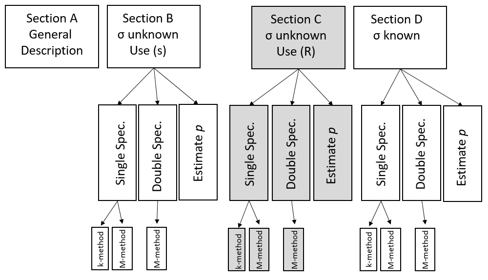
Figure 3.6 Content of MIL-STD-414
The function \(\verb!AAZ19()!\) in the R package \(\verb!AQLSchemes!\) can retrieve the normal, tightened or reduced sampling plans for the variability known or unknown cases from the ANSI/ASQ Z1.9 standard. This function eliminates the need to reference the tables, and provides the required sample size, the acceptability constant (k) and the maximum allowable proportion nonconforming (M). When given the sample data and the specification limits, the function \(\verb!EPn!\) in the same package can calculate the estimated proportion non-conforming from sample data as illustrated in section 3.2.
To illustrate the use of these functions, consider the example of the use of ANSI/ASQ Z1.9 on p. 163 of (Christensen, Betz, and Stein 2013). The minimum operating temperature for operation of a device is specified to be 180\(^{\circ}\)F and the maximum operating temperature is 209\(^{\circ}\)F. A lot size \(N =\) 40 is submitted for inspection with the variability unknown. The AQL is 1%, and the inspection level is II.
The function \(\verb!AAZ19()!\) has two required arguments, the first argument \(\verb!type!\), that can take on the values \(\verb!'Normal'!\), \(\verb!'Tightened'!\) or \(\verb!'Reduced'!\). It must be supplied to override the default value \(\verb!'Normal'!\). A second argument \(\verb!stype!\) can take on the values \(\verb!'unknown'!\) or \(\verb!'known'!\). It must be supplied to override the default value \(\verb!'unknown'!\). The function \(\verb!AAZ19()!\) is called in the same the way the functions \(\verb!AASingle()!\) and \(\verb!AADouble()!\) were called. They were illustrated in the last chapter.
The section of R code below illustrates the function call, the interactive queries and answers and the resulting plan. The second argument to the function \(\verb!AAZ19()!\) was left out to get the default value.
> library(AQLSchemes)
> AAZ19('Normal')

MIL-STD-414 ANSI/ASQ Z1.9

What is the Inspection Level?

1: S-3
2: S-4
3: I
4: II
5: III

Selection: 4

What is the Lot Size?

 1: 2-8                2: 9-15               3: 16-25              4: 26-50
 5: 51-90              6: 91-150             7: 151-280            8: 281-400
 9: 401-500           10: 501-1200          11: 1201-3200         12: 3201-10,000
13: 10,001-35,000     14: 35,001-150,000    15: 150,001-500,000   16: 500,001 and over


Selection: 4

What is the AQL in percent nonconforming per 100 items?

 1: 0.10   2: 0.15   3: 0.25   4: 0.40   5: 0.65   6: 1.0    7: 1.5    8: 2.5    9: 4.0
10: 6.5   11: 10

Selection: 6
     n           k        M
5.0000    1.524668   0.0333
The result shows that the sampling plan consists of taking a sample of 5 devices from the lot of 40 and comparing the estimated proportion non-conforming to 0.0333.
If the the operating temperatures of the 5 sampled devices (197,188,184,205, and 201), the \(\verb!EPn()!\) function can be called to calculate the estimated proportion non-conforming as shown in the R code below.
library(AQLSchemes)
sample<-c(197,188,184,205,201)
EPn(sample,sided="two",LSL=180,USL=209)
[1] 0.02799209
The argument \(\verb!sample!\) in the function call is the vector of sample data values. The argument \(\verb!sided!\) can be equal to \(\verb!"two"!\) or \(\verb!"one"!\), depending on whether there are double specification limits or a single specification limit. Finally, the arguments \(\verb!LSL!\) and \(\verb!USL!\) give the specification limits. If there is only a lower specification limit, change \(\verb!sided="two"!\) to \(\verb!sided="one"!\) and leave out \(\verb!USL!\). If there is only an upper specification limit leave out \(\verb!LSL!\) in addition to changing the value of \(\verb!sided!\).
The results of the function call indicate that the estimated proportion non-conforming is 0.02799209, which is less than the maximum tolerable proportion non-conforming = 0.0333; therefore the lot should be accepted as indicated on p. 163 of (Christensen, Betz, and Stein 2013). If the sample mean, sample standard deviation, and the sample size have already been calculated and stored in the variables \(\verb!xb!\), \(\verb!sd!\), and \(\verb!ns!\), then the function call can also be given as
The tightened sampling plan for the same inspection level, lot size, and AQL is found with the call:
Answering the queries the same way as shown above results in the plan:
Thus the lot would be rejected under tightened inspection since 0.02799209 > 0.0134.
The reduced sampling plan for the same inspection level, lot size and AQL is found with the call:
Answering the queries the same way as shown above results in the plan:
3.4 Gauge R&R Studies
Repeated measurements of the same part or process output do not always result in exactly the same value. This is called measurement error. It is necessary to estimate the variability in measurement error in order to determine if the measurement process is suitable. Gauge capability or Gauge R&R studies are conducted to estimate the magnitude of measurement error and partition this variability into various sources. The major sources of measurement error are repeatability and reproducibility. Repeatability refers to the error in measurements that occur when the same operator uses the gauge or measuring device to measure the same part or process output repeatedly. Reproducibility refers to the mesurment error that occurs due to different measuring conditions such as the operator making the measurement, or the environment where the measurement is made.
A basic gauge R&R study is conducted by having random sample of several operators measure each part or process output in a sample repeatedly. The operators are blinded as to which part they are measuring at the time they measure it.
The results of a gauge R&R study is shown in Table 3.1. In this study, there were three operators. The values represent the measurements of reducing sugar conentration in (g/L) of ten samples of the results of an enzymatic saccharification process for transforming food waste into fuel ethanol. Each operator measured each sample twice.
Table 3.1: Results of Gauge R&R Study
| Sample | Operator 1 | Operator 2 | Operator 3 |
|---|---|---|---|
| 1 | 103.24 | 103.16 | 102.96 |
| 2 | 103.92 | 103.81 | 103.76 |
| 3 | 109.13 | 108.86 | 108.70 |
| 4 | 108.35 | 108.11 | 107.94 |
| 5 | 105.51 | 105.06 | 104.84 |
| 6 | 106.63 | 106.61 | 106.60 |
| 7 | 109.29 | 108.96 | 108.84 |
| 8 | 108.76 | 108.39 | 108.23 |
| 9 | 108.03 | 107.86 | 107.72 |
| 10 | 106.61 | 106.32 | 106.21 |
| 1 | 103.56 | 103.26 | 103.01 |
| 2 | 103.86 | 103.80 | 103.75 |
| 3 | 109.23 | 108.79 | 108.75 |
| 4 | 108.29 | 108.24 | 107.99 |
| 5 | 105.53 | 105.11 | 104.80 |
| 6 | 106.65 | 106.57 | 106.55 |
| 7 | 109.28 | 109.12 | 109.03 |
| 8 | 108.72 | 108.43 | 108.27 |
| 9 | 108.11 | 107.84 | 107.79 |
| 10 | 106.77 | 106.23 | 106.13 |
An analysis of variance is used to to estimate \(\sigma^2_p\), the variance among different parts (or in this study samples); \(\sigma^2_o\), the variance among operators; \(\sigma^2_{po}\),the variance among part by operator; and \(\sigma^2_r\), the variance due to repeat measurments on one part by one operator. The gauge repeatability variance is defined to be \(\sigma^2_r\), and the gauge reproducibility variance is defined to be \(\sigma^2_o + \sigma^2_{po}\).
In the Rcode and output below, the measurement data from Table 3.1 are entered row by row into a single vector \(\verb!d!\), where operator changes fastest, sample second fastest, and the repeat measurements third. Next, the \(\verb!gageRRDesign()!\) function in the \(\verb!qualityTools!\) package is used to create the indicator variables for Operators, Parts, and Measurements in the design matrix \(\verb!gRR!\). The statement \(\verb!response(gRR)<-d!\) adds the measurment data in \(\verb!d!\) to the design , and the \(\verb!gageRR()!\) function produces the Analysis of Variance.
Below the Analysis of Variance are the estimates of: \(\sigma^2_r\) = 0.00478 (repeatability), \(\sigma^2_o\) = 0.03621 (Operator), \(\sigma^2_{po}\) = 0.00733 (Operator:Part), and \(\sigma^2_p\) = 4.47552 (Part to Part). The reproducibility is \(\sigma^2_o + \sigma^2_{po}\) = 0.04354. The measurement error variance is then \(\sigma^2_{gauge}\)=0.04832 (totalRR), which is the sum of the repeatability and reproducibility.
library(qualityTools)
design=gageRRDesign(Operators=3, Parts=10 ,
  Measurements=2, randomize=FALSE)
#set the response
response(design)=c(103.24,103.16,102.96,103.92,103.81,
                     103.76,109.13,108.86,108.70,108.35,
                     108.11,107.94,105.51,105.06,104.84,
                     106.63,106.61,106.60,109.29,108.96,
                     108.84,108.76,108.39,108.23,108.03,
                     107.86,107.72,106.61,106.32,106.21,
                     103.56,103.26,103.01,103.86,103.80,
                     103.75,109.23,108.79,108.75,108.29,
                     108.24,107.99,105.53,105.11,104.80,
                     106.65,106.57,106.55,109.28,109.12,
                     109.03,108.72,108.43,108.27,108.11,
                     107.84,107.79,106.77,106.23,106.13)
gA<-gageRR(design)
plot(gA)

AnOVa Table -  crossed Design
              Df Sum Sq Mean Sq  F value               Pr(>F)
Operator       2   1.49   0.744  155.740 < 0.0000000000000002 ***
Part           9 241.85  26.873 5627.763 < 0.0000000000000002 ***
Operator:Part 18   0.35   0.019    4.072             0.000346 ***
Residuals     30   0.14   0.005
---
Signif. codes:  0 ‘***’ 0.001 ‘**’ 0.01 ‘*’ 0.05 ‘.’ 0.1 ‘ ’ 1

----------

Gage R&R

---
 * Contrib equals Contribution in %
**Number of Distinct Categories (truncated signal-to-noise-ratio) = 13 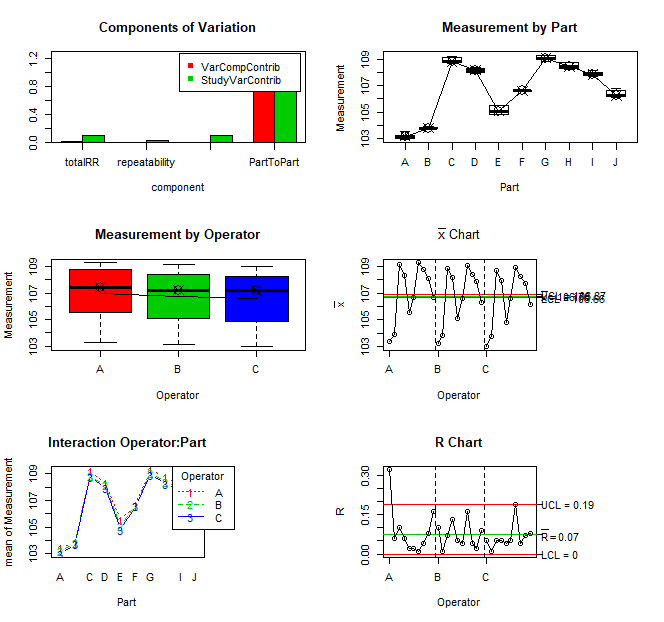
Figure 3.7 Gauge R&R Plots
The graph produced by the \(\verb!plot(gA)!\) statement can identify any outliers that may skew the results. From the boxplots in the upper right and middle left, it can be seen that variability of measurements on each part are reasonably consistent and operators are consistent with no apparent outliers.
From the plots on the top left and middle right, it can be seen that \(\sigma^2_{gauge}\) is small relative to the \(\sigma^2_p\). Generally, the gauge or measuring instrument is considered to be suitable if the process to tolerance \(P/T=\frac{6\times\sigma_{gauge}} {USL-LSL} \le 0.10\) where \(\sigma_{gauge}=\sqrt{\sigma^2_{gauge}}\) and \(USL\), and \(LSL\) are the upper and lower specification limits for the part being measured.
If the \(P/T\) ratio is greater than 0.1, looking at the \(\sigma^2_{repeatability}\) and \(\sigma^2_{reproducibility}\) gives some information about how to improve the measuring process. If \(\sigma^2_{repeatability}\) is the largest portion of measurment error it would indicate that the gauge or measuring device is inadequate since this variance represents the variance of repeat measurements of the same part by the same operator with the same gauge. If \(\sigma^2_{reproducibility}\) is the largest portion of measurement error, and if the plots on the middle and bottom left showed large variability in operator averages or inconsistent trends of measurments across parts for each operator, then perhaps better training of operators could reduce \(\sigma^2_o\) and \(\sigma^2_{po}\) therby reducing \(\sigma^2_{gauge}\).
3.5 Further Reading
Chapters 2 and 3 have presented an introduction to lot-by-lot attribute and variable sampling plans and AQL based attribute and variable sampling schemes. Additional sampling plans exist for rectification sampling, accept-on-zero sampling plans, and continuous sampling plans that are useful when there is a continuous flow of product that can’t naturally be grouped. Books by (Shmueli 2016) and (Schilling and Neubauer 2017) present more information on these topics.
Section 3.4 presented an introduction to measurement analysis. Again there is a more comprehensive coverage of this topic in (Burdick, Borror, and Montgomery 2005).
3.6 Summary
This chapter has discussed variables sampling plans and schemes. The major advantage to variables sampling plans over attribute plans is the same protection levels with reduced sample sizes. Table 3.1 (patterned after one presented by (Schilling and Neubauer 2017)) shows the average sample numbers for various plans that are matched to a single sampling plan for attributes with \(n=\) 50, \(c=\) 2. In addition to reduced sample sizes, variable plans provide information like the mean and estimated proportion defective below the lower specification limit and above the upper specification limit. This information can be valuable to the producer in correcting the cause of rejected lots and improving the process to produce at the AQL level or better.
Table 3.2: Average Sample Numbers for Various Plans
| Plan | Average Sample Number |
|---|---|
| Single Attributes | 50 |
| Double Attributes | 43 |
| Multiple Attributes | 35 |
| Variables (\(\sigma\) unknown) | 27 |
| Variables (\(\sigma\) known) | 12 |
When a continuous stream of lots is being sampled, the published schemes with switching rules are more appropriate. They provide better protection for producer and consumer at a reduced average sample number. The variables plans and published tables described in this chapter are based on the assumption that the measured characteristic is normally distributed.
That being said, the need for any kind of acceptance sampling is dependent on the consistency of the supplier’s process. If the supplier’s process is consistent (or in a state of statistical control) and is producing defects or nonconformities at a level that is acceptable to the customer, (Deming 1986) pointed out that no inspection is necessary or cost effective. On the other hand, if the supplier’s process is consistent but producing defects or nonconformities at a level that is too high for the customer to tolerate, 100% inspection should always be required. This is because the number (or proportion) nonconforming in a random sample from the lot is uncorrelated with the proportion non-conforming in the remainder of the lot. This can be demonstrated with the following simple example.
If the producer’s process is stable and producing 3% nonconforming and delivering lots of 200 items to the customer, then the sampling results using an attribute single sampling plan a sample size of \(n=\) 46 and an acceptance number of \(c=\) 3 can be simulated with the following R code. \(\verb!ps!\) represents the proportion defective in the sample, and \(\verb!pr!\) represents the proportion defective in the remainder of the lot.
# Lot size N=200 with an average 3% defective
p<-rbinom(50,200,.03)
r<-seq(1:50)
# This loop simulates the number non-conforming in a sample of 46
# items from each of the simulated lots
for (i in 1:length(p)) {
  r[i]<-rhyper(1,p[i],200-p[i],46)
}
# this statement calculates the proportion non-conforming in each lot
ps<-r/46
#This statement calculates the proportion non-conforming
pr<-(p-r)/154
# in the unsampled portion of each lot
plot(pr~jitter(ps,1),xlab='Proportion nonconforming in Sample of 46',
     ylab='Proportion nonconforming in remainder of Lot')
abline(h=(.03*46)/46,lty=2)
cor(ps,pr)
Figure 3.8 is a plot of the simulated proportion nonconforming in the sample of 46 versus the proportion nonconforming in the remainder of the lot of 200-46. It can be seen that there is no correlation. When the process is stable, rejecting lots with more than 3 defectives in the sample and returning them to the producer will not change the overall proportion of defects the customer is keeping.
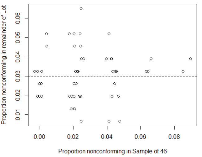
Figure 3.8 Simulated between the proportion nonconforming in a sample and the proportion nonconforming in the remainder of the lot
The same relationship will be true for attribute or variable sampling. This is exactly the reason that in 1980 Ford Motor Company demanded that their suppliers demonstrate their processes were in a state of statistical control with a proportion of nonconforming items at a level they could tolerate. Under those circumstances, no incoming inspection was necessary. Ford purchased a large enough share of their supplier’s output to make this demand. Following the same philosophy, the U.S. Department of Defense issued MIL-STD-1916 in 1996. This document stated that sampling inspection itself was an inefficient way of demonstrating conformance to the requirements of a contract, and that defense contractors should instead use process controls and statistical control methods. Again the large volume of supplies procured by the Department of Defense allowed them to make this demand of their suppliers. For smaller companies, who do not have that much influence on their suppliers, acceptance sampling of incoming lots may be the only way to assure themselves of adequate quality of their incoming components.
Chapter 4 will consider statistical process control and process improvement techniques that can help a company achieve stable process performance at an acceptable level of nonconformance. These methods should always be used when the producer is in-house. In cases where the producer is external to the customer, the use of sampling schemes like ANSI/ASQ-Z1.9 can encourage producers to work on making their processes more consistent with a low proportion of non-conformance. This is the case because a high or inconsistent level of nonconformance from lot to lot will result in a switch to tightened inspection using a sampling scheme. This increases the producer’s risk and the number of returned lots.
3.7 Exercises
Run all the code examples in the chapter, as you read.
Show that \((\overline{x}-LSL)/\sigma >k\) (the inequality in Equation 3.2), implies that \((\overline{x}-\mu_{RQL})/(\sigma/\sqrt{n}) > k\sqrt{n}+(LSL-\mu_{RQL})/(\sigma/\sqrt{n})\).
What is the distribution of \((\overline{x}-\mu_{RQL})/(\sigma/\sqrt{n})\), when \(x\) ~ \(N(\mu_{RQL}, \sigma)\)
The density of a plastic part used in a mobile phone is required to be at least 0.65g/cm\(^3\). The parts are supplied in lots of 5000. The AQL and LTPD are 0.01 and 0.05, and \(\alpha\)=.05, \(\beta\)=.10.
- Find an appropriate variables sampling plan (\(n\) and \(k\)) assuming the density is normally distributed with a known standard deviation \(\sigma\).
- Find an appropriate variables sampling plan assuming the standard deviation is unknown.
- Find an appropriate attributes sampling plan (\(n\) and \(c\)).
- Are the OC curves for the three plans you have found similar?
- What are the advantages and disadvantages of the variables sampling plan in this case.
A supplier of components to a small manufacturing company claims that they can send lots with no more than 1% defective components, but they have no way to prove that with past data. If they will agree to allow the manufacturing company to conduct inspection of incoming lots using an ANSI/ASQ-Z1.9 sampling scheme (and return rejected lots), how might this motivate them to be sure they can meet the 1% AQL?
The molecular weight of a polymer product should fall within \(LSL\)=2100 and \(USL\)=2350, the AQL=1%, and the RQL=8% with \(\alpha\) = 0.05, and \(\beta\) = 0.10. It is assumed to be normally distributed.
- Assuming the standard deviation is known to be \(\sigma\) = 60, find and appropriate variables sampling plan.
- Find the appropriate variables sampling plan for this situation if the standard deviation \(\sigma\) is unknown.
- If a sample of the size you indicate in (b) was taken from a lot and \(\overline{x}\) was found to be 2221, and the sample standard deviation \(s\) was found to be 57.2, would you accept or reject the lot?
- If the lot size is N=60, and the AQL=1.0%, use the \(\verb!AAZ19()!\) function to find the ANSI/ASQ Z1.9 sampling plan under Normal, Tightened, and Reduced inspection for the variability unknown case.
- Find the OC curves for the Normal and Tightened plans using the \(\verb!OCvar()!\) funtion in the \(\verb!AcceptanceSampling!\) package, and retrieve the OC values as shown in Section 3.1.2.2.
- Use the OC values for the Normal and Tightened plans and equations (??) and (??) in Chapter 2 to find the OC curve for the scheme that results from following the ANSI/ASQ Z1.9 switching rules.
- Plot all three OC curves on the same graph.
- If the specification limits were LSL=90, USL=130, and a sample of 7 resulted in the measurements: 123.13, 103.89, 117.93, 125.52, 107.79, 113.06, 100.19, would you accept or reject the lot under Normal inspection?
References
Burdick, R. K., Borror C. M., and D. C. Montgomery. 2005. Design and Analysis of Gauge R&R Studies. Philadelphia, PA: SIAM Society for Industrial; Applied Matematics.
Christensen, C., K. M. Betz, and M. S. Stein. 2013. The Certified Quality Process Analyst Handbook. 2nd ed. Milwaukee, Wisconsin: ASQ Quality Press.
Deming, W. E. 1986. Out of the Crisis. Cambridge, Mass.: MIT Center for Advance Engineering Study.
Lieberman, G. J., and G. J. Resnikoff. 1955. “Sampling Plans for Inspection by Variables.” Journal of the American Statistical Association 50: 467–516.
Mitra, A. 1998. Fundamentals of Quality Control and Improvement. Upper Saddle River, New Jersey: Prentice Hall.
Montgomery, D. C. 2013. Introduction to Statistical Quality Control. 7th ed. Hoboken, New Jersey: John Wiley & Sons.
Schilling, E. G., and D. V. Neubauer. 2017. Acceptance Sampling in Quality Control. 3rd ed. Boca Raton, Florida: Chapman; Hall/CRC.
Shmueli. 2016. Practical Acceptance Sampling - a Hands-on Guide. 2rd ed. Green Cove Springs, FL: Axelrod Schnall Piblishers.