Chapter 5 DoE for Troubleshooting and Improvement
5.1 Introduction
All work is performed within a system of interdependent processes. Components of processes include things such as people, machines, methods, materials, and the environment. This is true whether the work being performed provides a product through a manufacturing system, or a service.
Variation causes a system or process to provide something less than the desired result. The variation is introduced into the process by the components of the process as mentioned above. The variation from the ideal may be of two forms. One form is inconsistency or too much variation around the ideal output, and another is askew or off-target performance. Deming has often been quoted as having said “improving quality is all about reducing variability”.
The variability of process output can be classified into the two categories of: (1) assignable or special causes, and (2) common causes, as described in Chapter 4. The methods for effectively reducing common cause variability are much different than the methods for reducing variability due to assignable causes. The differences in the methods appropriate for reducing variability of each type are described next.
If process outputs are measured and plotted on control charts, assignable causes are identified by out-of-control signals. Usually the cause for an out-of-control signal on a Phase I Control Chart is obvious. Because out-of-control signals occur so rarely when a process is stable, examination of all the circumstances surrounding the specific time that an out-of-control signal occurred should lead to the discovery of unusual processing conditions which could have caused the problem. Tools such as the 5 W’s (who, what, where, when, and why), and ask why 5 times are useful in this respect.
Once the cause is discovered, a corrective action or adjustment should immediately be made to prevent this assignable cause from occurring again in the future. The efficacy of any proposed corrective action should be verified using a PDCA. This is a four step process. In the first step (plan) a proposed corrective action is described. In the second step (do) the proposed plan is carried out. In the third step (check) the effects of the corrective action are observed. If the action has corrected the problem proceed to the fourth step (act). In this step the corrective action is institutionalized by adding it to the OCAP described in Chapter 4, or implementing a preventative measure. If the corrective action taken in the third step did not correct the problem return to the first step (plan) and start again. The PDCA is often referred to as the Shewhart Cycle (who originally proposed it) or the Deming Cycle, since he strongly advocated it.
Common causes of variability cannot be recognized on a control chart, which would exhibit a stable pattern with points falling within the control limits with no unusual trends or patterns. Common causes don’t occur sporadically. They are always present. To discover common causes and create a plan to reduce their influence on process outputs requires careful consideration of the entire process, not just the circumstances immediately surrounding an out of control point.
Deming used his red bead experiment, and the funnel experiment to demonstrate the folly of blaming common cause problems on the immediate circumstances or people and then making quick adjustments. When the cause of less than ideal process outputs is due to common causes, quick adjustments are counter productive and could alienate the workforce and make them fearful to cooperate in discovering and reducing the actual causes of problems.
The way to reduce common cause variability is to study the entire process. In today’s environment of “Big Data” and Data Science, data analytics could be proposed as a way of studying the entire process and discovering ways to improve it. Through data analytics, past process information and outputs recorded in a quality information system(Burke and Silvestrini 2017) would be mined to discover relationships between process outputs and processing conditions. By doing this, it is felt that standardizing on the processing conditions that correlate with better process performance will improve the process.
However, this approach is rarely effective. The changes in process conditions to affect an improvement were usually unknown and not recorded in databases. Further, correlations found studying recorded data often do not represent cause and effect relationships. These correlations could be the result of cause and effect relations with other unrecorded variables.
A better way to study the entire process and find ways to improve is is through the use of a SIPOC (Britz et al. 2000) diagram (Suppliers provide Inputs that the Process translates to Outputs for the Customer) as shown in Figure 5.1. Here we can see that the output of a process is intended to satisfy or please the customer.
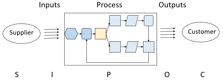
Figure 5.1 SIPOC Diagram
To discover changes necessary to counteract the influence of common causes and improve a process requires process knowledge and or intuition. When people knowledgeable about the process consider the inputs, processing steps, methods, and machines that translate the inputs to outputs, they can usually hypothesize potential reasons for excessive variation in outputs or off target performance. A list of potentially beneficial changes to the process can be gathered in brainstorming sessions. Affinity Diagrams, cause and effect diagrams, FMEA, and Fault Tree Analysis are useful ways for documenting ideas and opinions expressed in these sessions.
Once a list is developed, the potential changes can be tested during process operation. Again, the quote of George Box(Box 1966) is appropriate, “To find out what happens to a system (or process) when you interfere with it, you have to interfere with it not just passively observe it”. In this context, using data analytics, or attempting to discover potential process improvements by analyzing process variables stored in databases is what George Box means by passively observing a process. This method may not be successful because the changes needed to improve a process may have been unknown and not recorded in the databases. For this reason, correlations discovered in these exercises may not imply cause and effect relationships, and changes to the process based on these observed correlations might not lead to the anticipated process improvements.
To discover cause and effect relationships, changes must be made and the results of the changes must be observed. The PDCA approach is one way to test potential changes to a process. It is similar to the Edisonian technique of holding everything constant and varying one factor at a time to see if it causes a change to the process output of interest. This approach is popular in many disciplines, but it is not effective if changes in the process output are actually caused by simultaneous changes to more than one process factor. In addition, if a long list of potential changes to process factors to improve a process have been developed in a brainstorming session, it will be time consuming to test each one separately using the PDCA approach.
One method of simultaneously testing changes to several factors, and identifying joint (or interaction) effects between two or more factors is through use of a factorial experimental design. In a factorial design, all possible combinations of factor settings are tested. For example, if three process variables were each to be studied at four levels, there would be a total of \(4\times 4\times 4 = 4^3 = 64\) combinations tested. This seems like a lot of testing, but the number can usually be reduced by restricting the number of levels of each factor to two.
If the factor can be varied over a continuous range (like temperature), then the experimenter should choose two levels as far apart as reasonable to evoke a change in the response. If the factor settings are categorical (like method 1, method 2, … etc.), the experimenter can choose to study the two levels that he or she feels are most different. By this choice, the changes between these two factor levels would have the largest chance of causing a change in the process output. If no difference in the process output can be found between these two factor levels, the experimenter should feel comfortable that there are no differences between any of the potential factor levels.
Factorial experiments with all factors having two levels (often called two-level factorial designs or \(2^k\) designs) are very useful. Besides being able to detect simultaneous effects of several factors, they are simple, easy to set up, easy analyze, and their results are easy to communicate. These designs are very useful for identifying ways to improve a process. If a Phase I control chart shows that the process is stable and in control, but the capability index (PCR) is such that the customer need is not met, then experimentation with the process variables or redesigning the process must be done to find a solution. Use of a \(2^k\) experimental design is an excellent way to do this. These designs are also useful for trying to identifying the cause or remedy for an out of control situation that was not immediately obvious.
\(2^k\) designs require at least \(2^k\) experiments, and when there are many potential factors being studied, the basic two-level factorial designs still require a large number of experiments. This number can be drastically reduced using just a fraction of the total runs required for a \(2^k\) design, and fractional factorial, \(2^{k-p}\) designs, are again very useful for identifying ways to improve a process.
ISO (The International Standards Organization) Technical Committee 69 recognized the importance of \(2^k\), and \(2^{k-p}\) experimental designs and response surface designs for Six Sigma and other process improvement specialists, and they issued technical reports ISO/TC 29901 in 2007 and ISO/TR 12845 in 2010 (Johnson and Boulanger 2012). These technical reports were guideline documents. ISO/TC 29901 offered a template for implementation of \(2^k\) experimental designs for process improvement studies, and ISO/TR 12845 a template for implementation of \(2^{k-p}\) experimental designs for process improvement studies.
Although \(2^k\)experiments are easy to set up, analyze, and interpret, they require too many experiments if there are 5 or 6 factors or more. While \(2^{k-p}\) designs require many fewer experiments, the analysis is not always so straight forward, especially for designs with many factors. Other experimental design plans such as the Alternative Screening Designs in 16 runs(Jones and Montgomery 2010), and the Definitive Screening Designs (Jones and Nachtsheim 2011), can handle a large number of factors yet offer reduced run size and straightforward methods of analysis, using functions in the R package \(\verb!daewr!\). The Definitive Screening designs allow three-level factors and provide the ability to explore curvalinear response surface type models that the ISO Technical Committee 69 also recognized as important for process improvement studies.
After some unifying definitions, this chapter will discuss \(2^k\) designs and fractions of \(2^k\) designs, Alternative Screening designs, and Definitive Screening designs and provide examples of creating and analyzing data from all of these using R.
5.2 Definitions:
An Experiment (or run) is conducted when the experimenter changes at least one of the factor levels he or she is studying (and has control over) and then observes the result, i.e., do something and observe the result. This is not the same as passive collection of observational data.
Experimental Unit is the item under study upon which something is changed. This could be human subjects, raw materials, or just a point in time during the operation of a process.
Treatment Factor (or independent variable) is one of the variables under study that is being controlled near some target value, or level, during any experiment. The level is being changed in some systematic way from run to run in order to determine the effect the change has on the response.
Lurking Variable (or Background variable) is a variable that the experimenter is unaware of or cannot control, but it does have an influence on the response. It could be an inherent characteristic of the experimental units (which are not identical) or differences in the way the treatment level is applied to the experimental unit, or the way the response is measured. In a well-planned experimental design the effect of these lurking variables should balance out so as to not alter the conclusions.
Response (or Dependent Variable) is the characteristic of the experimental units that is measured at the completion of each experiment or run. The value of the response variable depends on the settings of the independent variables (or factor levels) and the lurking variables.
Factor Effect is the difference in the expected value or average of all potential responses at the high level of a factor and the expected value or average of all potential responses at the low level of a factor. It represents the expected change in the response caused by changing the factor from its low to high level. Although this effect is unknown, it can be estimated as the difference in sample average responses calculated with data from experiments.
Interaction Effect If there is an interaction effect between two factors, then the effect of one factor is different depending on the level of the other factor. Other names for an interaction effect are joint effect or simultaneous effect. If there is an interaction between three factors (called a three-way interaction), then the effect of one factor will be different depending on the combination of levels of the other two factors. Four-factor interactions and higher order interactions are similarly defined.
Replicate runs are two or more experiments with the same settings or levels of the treatment factors, but using different experimental units. The measured response for replicate runs may be different due to changes in lurking variables or the inherent characteristics of the experimental units.
Duplicates refers to duplicate measurements of the same experimental unit from one run or experiment. Differences in the measured response for duplicates is due to measurement error and these values should be averaged and not treated as replicate runs in the analysis of data.
Experimental Design is a collection of experiments or runs that is planned in advance of the actual execution. The particular experiments chosen to be part of an experimental design will depend on the purpose of the design.
Randomization is the act of randomizing the order that experiments in the experimental design are completed. If the experiments are run in an order that is convenient to the experimenter rather than in a random order, it is possible that changes in the response that appear to be due to changes in one or more factors may actually be due to changes in unknown and unrecorded lurking variables. When the order of experimentation is randomized, this is much less likely to occur due to the fact that changes in factors occur in a random order that is unlikely to correlate with changes in lurking variables.
Confounded Factors results when changes in the level of one treatment factor in an experimental design correspond exactly to changes in another treatment factor in the design. When this occurs, it is impossible to tell which of the confounded factors caused a difference in the response.
Biased Factor results when changes in the level of one treatment factor, in an experimental design, correspond exactly to changes in the level of a lurking variable. When a factor is biased, it is impossible to tell if any resulting changes in the response that occur between runs or experiments is due to changes in the biased factor or changes in the lurking variable.
Experimental error is the difference in observed response for one particular experiment and the long run average response for all potential experimental units that could be tested at the same factor settings or levels.
5.3 \(2^k\) Designs
\(2^k\) designs have \(k\) factors each studied at 2 levels. Figure 5.2 shows an example of a \(2^3\) design (i.e., \(k=3\)). There are a total of \(2\times2\times2=8\) runs in this design. They represent all possible combinations of the low and high levels for each factor. In this figure the factor names are represented as A, B, and C, and the low and high levels of each factor are represented as \(-\) and \(+\), respectively. The list of all runs is shown on the left side of the figure where the first factor (A) alternates between low and high levels for each successive pair of runs. The second factor (B) alternates between pairs of low and high levels for each successive group of four runs, and finally the last factor (C) alternates between groups of four consecutive low levels and four consecutive high levels for each successive group of eight runs. This is called the standard order of the experiments.
The values of the response are represented symbolically as \(y\) with subscripts representing the run in the design. The right side of the figure shows that each run in the design can be represented graphically as the corners of a cube. If there are replicate runs at each of the 8 combination of factor levels, the responses (\(y\)) in the figure could be replaced by the sample averages of the replicates (\(\overline{y}\)) at each factor level combination.
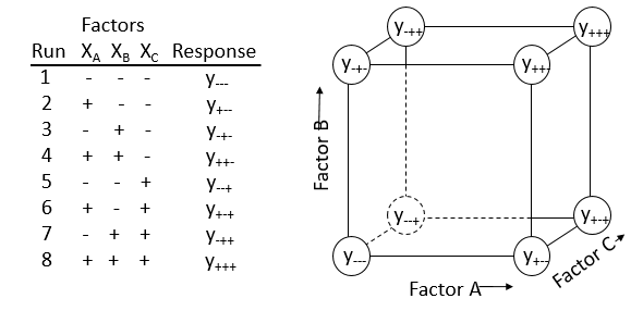
Figure 5.2 Symbolic representation of a \(2^3\) Design
With the graphical representation in Figure 5.2, it is easy to visualize the estimated factor effects. For example, the effect of factor A is the difference in the average of the responses on the right side of the cube (where factor A is at its high level) and the average of the responses on the left side of the cube. This is illustrated in Figure 5.3.
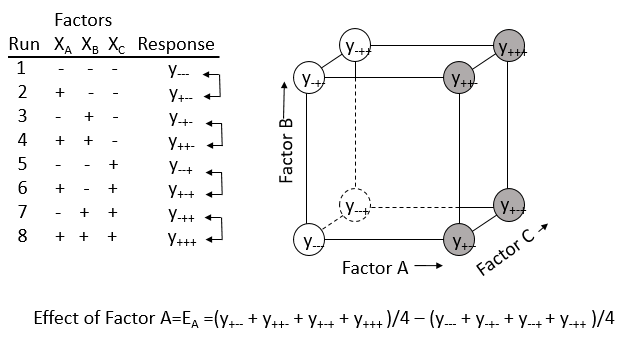
Figure 5.3 Representation of the Effect of Factor A
The estimated effect of factor B can be visualized similarly as the difference in the average of the responses at the top of the cube and the average of the responses at the bottom of the cube. The estimated effect of factor C is the difference in the average of the responses on the back of the cube and the average of the responses at the front of the cube.
In practice the experiments in a \(2^k\) design should not be run in the standard order, as shown in Figure 5.1. If that were done, any changes in a lurking variable that occurred near midway through the experimentation would bias factor C. Any lurking variable that oscillated between two levels could bias factors A or B. For this reason experiments are always run in a random order, once the list of experiments is made.
If the factor effects are independent, then the average response at any combination of factor levels can be predicted with the simple additive model
\[\begin{equation} y=\beta_0 + \beta_A X_A + \beta_B X_B + \beta_C X_C. \tag{5.1} \end{equation}\]
Where \(\beta_0\) is the grand average of all the response values; \(\beta_A\) is half the estimated effect of factor A (i.e., \(E_A/2\)); \(\beta_B\) is half the estimated effect of factor B; and \(\beta_C\) is half the estimated effect of factor C. \(X_A\), \(X_B\), and \(X_C\) are the \(\pm\) coded and scaled levels of the factors shown in Figure 5.1 and 5.2. The conversion between actual factor levels and the coded and scaled factor levels are accomplished with a coding and scaling equation like:
\[\begin{equation} X_A=\frac{\mbox{Factor level}-\left(\frac{\mbox{High level}+\mbox{Low level}}{2}\right)}{\left(\frac{\mbox{High level}-\mbox{Low level}}{2}\right).} \tag{5.2} \end{equation}\]
This coding and scaling equation converts the high factor level to \(+1\), the low factor level to \(-1\), and factor levels between the high and low to a value between \(-1\) and \(+1\). When a factor has qualitative levels like: Type A, or Type B. One level is designated as \(+1\) and the other as \(-1\). In this case predictions from the model can only be made at these two levels of the factor.
If the factor effects are dependent, then effect of one factor is different at each level of another factor or each combination of levels of other factors. For example the estimated conditional main effect of factor B, calculated when factor C is held constant at its low level is
(\(E_{B|C=-}=(y_{-+-}+y_{++-})/2-(y_{---}+y_{+--})/2\)).
This can be visualized as the difference in the average of the two responses in the gray circles at the top front of the cube on the left side of Figure 5.4 and the average of the two responses in the gray circles at the bottom front of the cube shown on the left side of Figure 5.4. The estimated conditional main effect of factor B when factor C is held constant at its high level is
(\(E_{B|C=+}=(y_{-++}+y_{+++})/2-(y_{--+}+y_{+-+})/2\)).
It can be visualized on the right side of Figure 5.4 as the difference of the average of the two responses in the gray circles at top back of the cube and the average of the two responses in the gray circles at the back bottom of the cube.
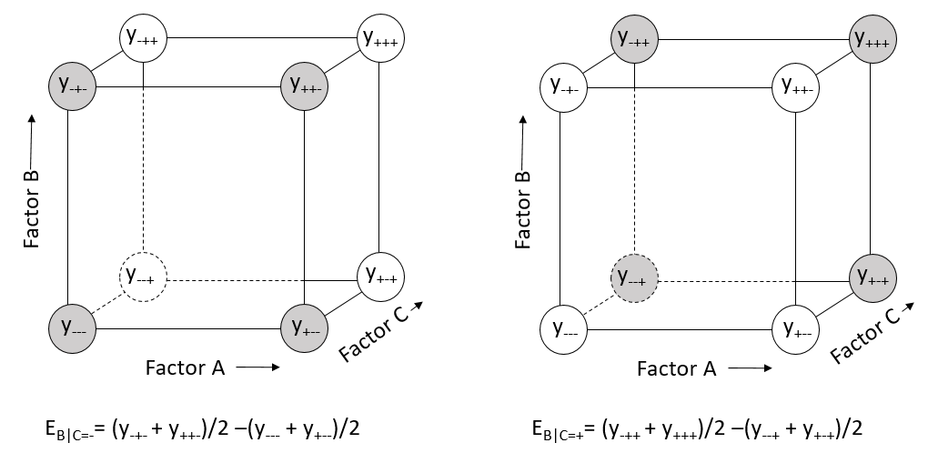
Figure 5.4 Conditional Main Effects of B given the level of C
The B\(\times\)C interaction effect is defined as half the difference in the two estimated conditional main effects as shown in Equation (5.3).
\[\begin{align} E_{BC}&=(E_{B|C=+} - E_{B|C=-})/2\\ &=(y_{-++}+y_{+++}+y_{---}+y_{+--})/4)-(y_{-+-}+y_{++-}+y_{--+}+y_{+-+})/4 \tag{5.3} \end{align}\]
Again this interaction effect can be seen to be the difference in the average of the responses in the gray circles and the average of the responses in the white circles shown in Figure 5.5.
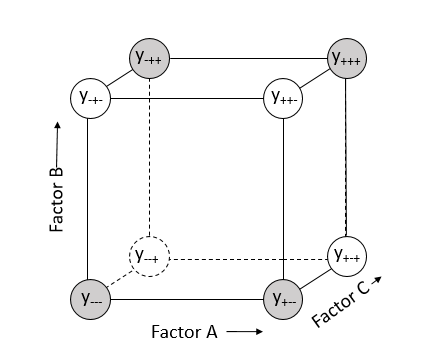
Figure 5.5 BC interaction effect
If the interaction effect is not zero, then additive model in Equation (5.1) will not be accurate. Adding half of the estimated interaction effect to model (5.1) results in model (5.4) which will have improved predictions if the effect of factor B is different depending on the level of Factor C, or the effect of Factor C is different depending on the level of factor B.
\[\begin{equation} y=\beta_0 + \beta_A X_A + \beta_B X_B + \beta_C X_C +\beta_{BC} X_B X_C \tag{5.4} \end{equation}\]
Each \(\beta\) coefficient in this model can be calculated as half the difference in two averages, or by fitting a multiple regression model to the data. If there are replicate responses at each of the eight combinations of factor levels (in the \(2^3\) design shown in Figure 5.1) then significance tests can be used to determine which coefficients (i.e., \(\beta\)s) are significantly different from zero. To do that, start with the full model:
\[\begin{align} y=&\beta_0 + \beta_A X_A + \beta_B X_B + \beta_C X_C\\ +&\beta_{AB} X_A X_B + \beta_{AC} X_A X_C + \beta_{BC} X_B X_C + \beta_{ABC} X_A X_B X_C. \tag{5.5} \end{align}\]
The full model can be extended to \(2^k\) experiments as shown in Equation (5.6).
\[\begin{equation} y=\beta_0 + \sum_{i=1}^k \beta_i X_i +\sum_{i=1}^k\sum_{j \ne i}^k \beta_{ij} X_i X_j +\cdots +\beta_{i\cdots k}X_i \cdots X_k. \tag{5.6} \end{equation}\] Any insignificant coefficients found in the full model can be removed to reach the final model.
5.3.1 Examples
In this section two examples of \(2^k\) experiments will used to illustrate the R code to design, analyze, and interpret the results.
5.3.2 Example 1: A \(2^3\) Factorial in Battery Assembly
A \(2^3\) experiment was used to study the process of assembling nickel-cadmium batteries. This example is taken from Ellis Ott’s book Process Quality Control-Troubleshooting and Interpretation of Data (Ott 1975).
Nickel-Cadmium batteries were assembled with the goal of having a consistently high capacitance. However much difficulty was encountered in during the assembly process resulting in excessive capacitance variability. A team was organized to find methods to improve the process. This is an example of a common cause problem. Too much variability all of the time.
While studying the entire process as normally would be done to remove a common cause problem, the team found that two different production lines in the factory were used for assembling the batteries. One of these production lines used a different concentration of nitrate than the other line. They also found that two different assembly lines were used in the factory. One line was using a shim in assembling the batteries and the other line did not. In addition, two processing stations were used in the factory; at one station, fresh hydroxide was used, while reused hydroxide was used in the second station. The team conjectured that these differences in the assembly could be the cause of the extreme variation in the battery capacitance. They decided it would be easy to set up a \(2^3\) experiment varying the factor levels shown in Table 5.1, since they were already in use in the factory.
Table 5.1 Factors and Levels in Nickel-Cadmium Battery Assembly Experiment
| Factors | Level (-) | Level (+) |
|---|---|---|
| A–Production line | 1=low level of nitrate | 2=high level of nitrate |
| B–Assembly line | 1-using shim in assembly | 2=no shim used in assembly |
| C–Processing Station | 1-using fresh hydroxide | 2=using reused hydroxide |
The team realized that if they found differences in capacitance caused by the two different levels of factor A, then the differences may have been caused by either differences in the level of nitrite used, or other differences in the two production lines, or both. If they found a significant effect of factor A, then further experimentation would be necessary to isolate the specific cause. A similar situation existed for both factors B and C. A significant effect of factor B could be due to whether a shim was used in assembly or due to other differences in the two assembly lines. Finally, a significant effect of factor C could be due to differences in the two processing stations or caused by the difference in the fresh and reused hydroxide.
Table 5.2 shows the eight combinations of coded factor levels and the responses for six replicate experiments or runs conducted at each combination. The capacitance values were coded by subtracting the same constant from each value (which will not affect the results of the analysis). The actual experiments were conducted in a random order so that any lurking variables like properties of the raw materials would not bias any of the estimated factor effects or interactions. Table 5.2 is set up in the standard order of experiments that was shown in Figure 5.1.
Table 5.2 Factor Combinations and Response Data for Battery Assembly Experiment
| \(X_A\) | \(X_B\) | \(X_C\) | Capacitance | ||||||
|---|---|---|---|---|---|---|---|---|---|
| \(-\) | \(-\) | \(-\) | \(-0.1\) | 1.0 | 0.6 | \(-0.1\) | \(-1.4\) | 0.5 | |
| \(+\) | \(-\) | \(-\) | 0.6 | 0.8 | 0.7 | 2.0 | 0.7 | 0.7 | |
| \(-\) | \(+\) | \(-\) | 0.6 | 1.0 | 0.8 | 1.5 | 1.3 | 1.1 | |
| \(+\) | \(+\) | \(-\) | 1.8 | 2.1 | 2.2 | 1.9 | 2.6 | 2.8 | |
| \(-\) | \(-\) | \(+\) | 1.1 | 0.5 | 0.1 | 0.7 | 1.3 | 1.0 | |
| \(+\) | \(-\) | \(+\) | 1.9 | 0.7 | 2.3 | 1.9 | 1.0 | 2.1 | |
| \(-\) | \(+\) | \(+\) | 0.7 | \(-0.1\) | 1.7 | 1.2 | 1.1 | \(-0.7\) | |
| \(+\) | \(+\) | \(+\) | 2.1 | 2.3 | 1.9 | 2.2 | 1.8 | 2.5 |
The design can be constructed in standard order to match the published data using the \(\verb!fac.design()!\) and \(\verb!add.response()!\) functions in the R package \(\verb!DoE.Base!\) as shown in the section of code below.
library(DoE.base)
design<-fac.design(nlevels=c(2,2,2),replications=6,randomize=F,
                   factor.names=list(A=c("nitrate-1", "nitrate-2"),B=c("Shim","No Shim"),
                                     C=c("Fresh","Reused")))
Capacitance<-c( -.1,  .6,  .6, 1.8, 1.1, 1.9,  .7, 2.1,
                1.0,  .8, 1.0, 2.1,  .5,  .7, -.1, 2.3,
                .6,  .7,  .8, 2.2,  .1, 2.3, 1.7, 1.9,
                -.1, 2.0, 1.5, 1.9,  .7, 1.9, 1.2, 2.2,
                -1.4,  .7, 1.3, 2.6, 1.3, 1.0, 1.1, 1.8,
                .5,  .7, 1.1, 2.8, 1.0, 2.1, -.7, 2.5)
add.response(design,Capacitance)
The R function \(\verb!lm()!\) can be used to fit the full model (Equation (5.4)) by least-squares regression analysis to the data from the experiment using the code below. Part of the output is shown below the code.
mod1<-lm(Capacitance~A*B*C, data=design)
summary(mod1)

Coefficients:
            Estimate Std. Error t value Pr(>|t|)
(Intercept)  1.18750    0.08434  14.080  < 2e-16 ***
A1           0.54583    0.08434   6.472 1.03e-07 ***
B1           0.32917    0.08434   3.903 0.000356 ***
C1           0.11667    0.08434   1.383 0.174237
A1:B1        0.12083    0.08434   1.433 0.159704
A1:C1        0.04167    0.08434   0.494 0.623976
B1:C1       -0.24167    0.08434  -2.865 0.006607 **
A1:B1:C1     0.03333    0.08434   0.395 0.694768
Signif. codes:  0 ‘***’ 0.001 ‘**’ 0.01 ‘*’ 0.05 ‘.’ 0.1 ‘ ’ 1

Residual standard error: 0.5843 on 40 degrees of freedom
Multiple R-squared:  0.6354,	Adjusted R-squared:  0.5715
F-statistic: 9.957 on 7 and 40 DF,  p-value: 3.946e-07
In the output, it can be seen that factor A and B are significant as well as the two-factor interaction BC. There is a positive regression coefficient for factor A. Since this coefficient is half the effect of A=(production line or level of nitrate) it means that a higher average capacitance is expected using production line 2 where the high concentration of nitrate was used.
Because there is a significant interaction of factors B and C, the main effect of factor B cannot be interpreted in the same way as the main effect for factor A. The significant interaction means the conditional effect of factor B=(Assembly line or use of a shim) is different depending on the level of factor C=(Processing station and fresh or reused hydroxide). The best way to visualize the interaction is by using an interaction plot. The R function \(\verb!interaction.plot()!\) is used in the section of code below to produce the interaction plot shown in Figure 5.6.
Assembly<-design$B
Hydroxide<-design$C
interaction.plot(Assembly,Hydroxide,Capacitance,type="b",pch=c(1,2),col=c(1,2),data=design)
In this figure it can be seen that the effect of using a shim in assembly reduces the capacitance by a greater amount when fresh hydroxide at processing station 1 is used than when reused hydroxide at processing station 2 is used. However, the highest expected capacitance of the assembled batteries is predicted to occur when using fresh hydroxide and assembly line 1 where no shim was used.
The fact that there was an interaction between assembly line and processing station, was at first puzzling to the team. This caused them to further investigate and resulted in the discovery of specific differences in the two assembly lines and processing stations. It was conjectured that standardizing the two assembly lines and processing stations would improve the battery quality by making the capacitance consistently high. A pilot run was made to check, and the results confirmed the conclusions of the \(2^3\) design experiment.
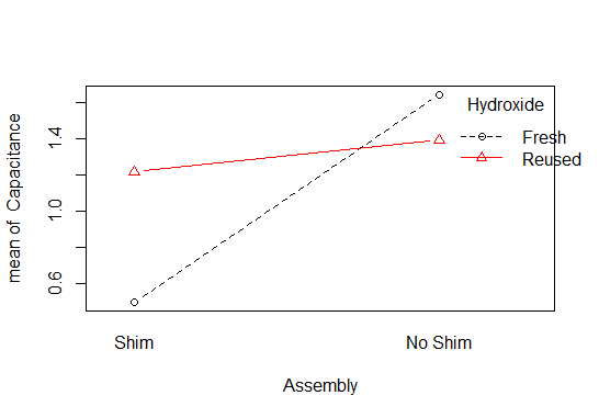
Figure 5.6 BC Interaction Plot
The assumptions required for a least-squares regression fit are that the variability in the model residuals (i.e., actual minus model predictions) should be constant across the range of predicted values, and that the residuals should be normally distributed. Four diagnostic plots for checking these assumptions can be easily made using the code below, and are shown in Figure 5.7.
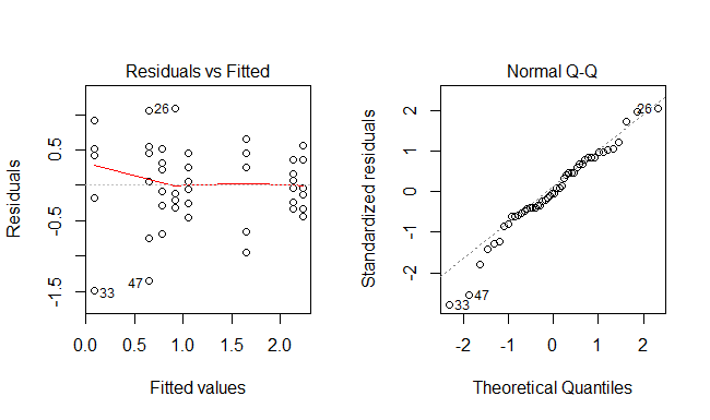
Figure 5.7 Model Diagnostic Plots
The plot on the left indicates the spread in the residuals is approximately equal for each of the predicted values. If the spread in the residuals increased noticeably as the fitted values increased it would indicate that a more accurate model could be obtained by transforming the response variable before using the \(\verb!lm()!\) function see (Lawson 2015) for examples. The plot on the right is a normal probability plot of the residuals. Since the points fall basically along the diagonal straight line it indicates the normality assumption is satisfied. To understand how far from the straight line the points may lie before indicating the normality assumption is contradicted, you can make repeated normal probability plots of randomly generated data using the commands:
5.3.3 Example 2: Unreplicated \(2^4\) Factorial in Injection Molding
The second example from (Durakovic 2017) illustrates the use of a \(2^4\) factorial, with only one replicate of each of the 16 treatment combinations. The purpose of the experiments was to improve the quality of injection-molded parts by reducing the excessive flash. This is again a common cause that makes the average flash excessive (off target). The factors that were under study and their low and high levels are shown in Table 5.3.
Table 5.3 Factors and Levels for Injection Molding Experiment
| Factors | Level (-) | Level (+) |
|---|---|---|
| A-Pack Pressure in Bar | 10 | 30 |
| B–Pack Time in sec. | 1 | 5 |
| C–Injection Speed mm/sec | 12 | 50 |
| D–Screw Speed in rpm | 100 | 200 |
A full factorial design and the observed flash size for each run are shown in Table 5.4. This data is in standard order (first column changing fastest etc.) but the experiments were again run in random order.
Table 5.4 Factor Combinations and Response Data for Injection Molding Experiment
| \(X_A\) | \(X_B\) | \(X_C\) | \(X_D\) | Flash(mm) |
|---|---|---|---|---|
| \(-\) | \(-\) | \(-\) | \(-\) | 0.22 |
| \(+\) | \(-\) | \(-\) | \(-\) | 6.18 |
| \(-\) | \(+\) | \(-\) | \(-\) | 0.00 |
| \(+\) | \(+\) | \(-\) | \(-\) | 5.91 |
| \(-\) | \(-\) | \(+\) | \(-\) | 6.60 |
| \(+\) | \(-\) | \(+\) | \(-\) | 6.05 |
| \(-\) | \(+\) | \(+\) | \(-\) | 6.76 |
| \(+\) | \(+\) | \(+\) | \(-\) | 8.65 |
| \(-\) | \(-\) | \(-\) | \(+\) | 0.46 |
| \(+\) | \(-\) | \(-\) | \(+\) | 5.06 |
| \(-\) | \(+\) | \(-\) | \(+\) | 0.55 |
| \(+\) | \(+\) | \(-\) | \(+\) | 4.84 |
| \(-\) | \(-\) | \(+\) | \(+\) | 11.55 |
| \(+\) | \(-\) | \(+\) | \(+\) | 9.90 |
| \(-\) | \(+\) | \(+\) | \(+\) | 9.90 |
| \(+\) | \(+\) | \(+\) | \(+\) | 9.90 |
In the R code below, the \(\verb!FrF2()!\) function in the R package \(\verb!FrF2()!\) is used to create this design. Like the design in Example 1, it was created in standard order using the argument \(\verb!randomize=F!\) in the \(\verb!FrF2!\) function call. This was to match the already collected data shown in Table 5.4. When using the \(\verb!fac.design()!\) or \(\verb!FrF2()!\) function to create a data collection form prior to running experiments, the argument \(\verb!randomize=F!\) should be left out and the default will create a list of experiments in random order. The random order will minimize the chance of biasing any estimated factor effect with the effect of any lurking variable that may change during the course of running the experiments.
library(FrF2)
design2<-FrF2(16,4,factor.names=list(A=c(10,30),B=c(1,5),C=c(12,50),D=c(100,200)),
              randomize=F)
Flash<-c(.22,6.18,0,5.91,6.6,6.05,6.76,8.65,0.46,5.06,0.55,4.84,11.55,9.9,9.9,9.9)
add.response(design2,Flash)
The R function \(\verb!lm()!\) can be used to calculate the estimated regression coefficients for the full model (Equation (5.6) with \(k=4\)). However, the \(\verb!Std. Error!\), \(\verb!t value!\), and \(\verb!Pr(>|t|)!\) shown in the output for the first example cannot be calculated because there were no replicates in this example.
Graphical methods can be used to determine which effects or coefficients are significantly different from zero. If all the main effects and interactions in the full model were actually zero, then all of the estimated effects or coefficients would only differ from zero by an approximately normally distributed random error (due to the central limit theorem). If a normal probability plot were made of all the estimated effects or coefficients, any truly nonzero effects should appear as outliers on the probability plot.
The R code below shows the use of the R function \(\verb!lm()!\) to fit the full model to the data, and a portion of the output is shown below the code.
mod2<-lm(Flash~A*B*C*D, data=design2)
summary(mod2)

Coefficients:
             Estimate Std. Error t value Pr(>|t|)
(Intercept)  5.783125         NA      NA       NA
A1           1.278125         NA      NA       NA
B1           0.030625         NA      NA       NA
C1           2.880625         NA      NA       NA
D1           0.736875         NA      NA       NA
A1:B1        0.233125         NA      NA       NA
A1:C1       -1.316875         NA      NA       NA
B1:C1        0.108125         NA      NA       NA
A1:D1       -0.373125         NA      NA       NA
B1:D1       -0.253125         NA      NA       NA
C1:D1        0.911875         NA      NA       NA
A1:B1:C1     0.278125         NA      NA       NA
A1:B1:D1    -0.065625         NA      NA       NA
A1:C1:D1    -0.000625         NA      NA       NA
B1:C1:D1    -0.298125         NA      NA       NA
A1:B1:C1:D1 -0.033125         NA      NA       NA

Residual standard error: NaN on 0 degrees of freedom
Multiple R-squared:      1,	Adjusted R-squared:    NaN
F-statistic:   NaN on 15 and 0 DF,  p-value: NA
The function \(\verb!fullnormal()!\) from the \(\verb!daewr!\) package can be used to make a normal probability plot of the coefficients (Figure 5.8) as shown in the code below.
The argument \(\verb!coef(mod2)[-1]!\) requests a normal probability plot of the 15 coefficients in \(\verb!mod2!\) (excluding the first term which is the intercept).
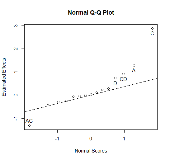
Figure 5.8 Normal Plot of Coefficients
In this plot it can be seen that main effects A=Pack Pressure in Bar, C=Injection Speed in mm/sec, and D=Screw Speed in rpm all appear to be significant since they do not fall along the straight line of insignificant effects. All three of these significant factors have positive coefficients which, would lead one to believe that setting all three of these factors to their low levels would minimize flash and improve the quality of the injected molded parts.
However, the CD interaction and the AC interaction also appear to be significant. Therefore, these two interaction plots should be studied before drawing any final conclusions. The R code to make these two interaction plots (Figures 5.9 and 5.10) is shown below.
A_Pack_Pressure<-design2$A
C_Injection_Speed<-design2$C
D_Screw_Speed<-design2$D
interaction.plot(A_Pack_Pressure,C_Injection_Speed,Flash,type="b",
                 pch=c(1,2),col=c(1,2))
interaction.plot(C_Injection_Speed,D_Screw_Speed,Flash,type="b",
                 pch=c(1,2),col=c(1,2))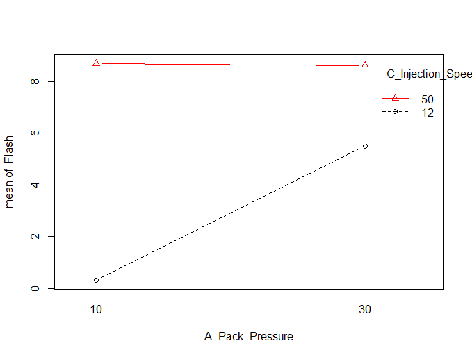
Figure 5.9 AC Interaction Plot
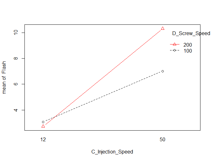
Figure 5.10 CD Interaction Plot
In Figure 5.9 it can be seen that factor A: Pack pressure only has a positive effect when factor C: Injection speed is set to its low level (12mm/sec). In Figure 5.10 it can be seen that the effect of Factor C: Injection speed is much stronger when Factor D: Screw speed is set to its high value of 200 RPM. Therefore the final recommendation was to run the injection molding machine at the low levels of Factor A (Pack Pressure=10 Bar), the low level of Factor C (Injection Speed=12 mm/sec) and the high level of Factor D (Screw Speed=200 rpm ).
Factor B (Pack Time) was not significant nor was there any significant interaction involving Factor B. Therefore, this factor can be set to the level that is least expensive.
In the article (Durakovic 2017), the reduced model involving main effects A, C, D and the AC and CD interactions was fit to the data and the normal plot of residuals and residuals by predicted values showed that the least squares assumptions were satisfied and that the predictions from this model would be accurate.
In both of the examples shown in this section, discovering significant interactions was key to solving the problem. In the real world, factor effects are rarely independent, and interactions are common. Therefore, if many factors are under study it would be better to study all of the factors jointly in an experimental design, so that all potential interactions could be detected.
For example, if 6 factors were under study it would be better to study all factors simultaneously in a \(2^{6}\) factorial experiment than it would to study the first three factors in a \(2^3\) factorial experiment and the remaining three factors in another \(2^3\) factorial experiment. When running two separate \(2^3\) designs it would be impossible to detect interactions between any of the factors studied in the first experiment and any of the factors studied in the second experiment.
After brainstorming sessions where cause-and-effect diagrams are produced, there are often many potential factors to be investigated. However, the number of experiments required for a \(2^k\) factorial experiment is \(2^k\). This can be large, for example 64 experiments are required for a \(2^6\) factorial and 1024 experiments required for a \(2^{10}\) factorial.
Fortunately, many of the advantages obtained by running a \(2^k\) full factorial can be obtained by running just a fraction of the total \(2^k\) experiments. The next section will illustrate how to create a fraction of a \(2^k\) design and examples will be used to show how the results can be interpreted.
5.4 \(2^{k-p}\) Fractional Factorial Designs
5.4.1 One-Half Fraction Designs
When creating a fraction of a \(2^k\) factorial, the runs or experiments chosen to be in the fraction must be selected strategically. Table 5.5 shows what happens if the runs in a one-half fraction are not selected strategically. The left side of the table shows a \(2^4\) design in standard order. The column labeled “k-e” is an indicator of whether the run should be kept or eliminated from the fraction of the \(2^4\) design. The runs to be eliminated were chosen by a random selection process. The right side of the table shows the eight runs remaining in the one-half fraction after eliminating the runs with a “e” in the “k-e” column.
Table 5.5 Fractional Factorial by random elimination
| k-e | run | A | B | C | D | run | A | B | C | D | |
|---|---|---|---|---|---|---|---|---|---|---|---|
| k | 1 | \(-\) | \(-\) | \(-\) | \(-\) | 1 | \(-\) | \(-\) | \(-\) | \(-\) | |
| e | 2 | \(+\) | \(-\) | \(-\) | \(-\) | 4 | \(+\) | \(+\) | \(-\) | \(-\) | |
| e | 3 | \(-\) | \(+\) | \(-\) | \(-\) | 5 | \(-\) | \(-\) | \(+\) | \(-\) | |
| k | 4 | \(+\) | \(+\) | \(-\) | \(-\) | 8 | \(+\) | \(+\) | \(+\) | \(-\) | |
| k | 5 | \(-\) | \(-\) | \(+\) | \(-\) | 10 | \(+\) | \(-\) | \(-\) | \(+\) | |
| e | 6 | \(+\) | \(-\) | \(+\) | \(-\) | 12 | \(+\) | \(+\) | \(-\) | \(+\) | |
| e | 7 | \(-\) | \(+\) | \(+\) | \(-\) | 13 | \(-\) | \(-\) | \(+\) | \(+\) | |
| k | 8 | \(+\) | \(+\) | \(+\) | \(-\) | 16 | \(+\) | \(+\) | \(+\) | \(+\) | |
| e | 9 | \(-\) | \(-\) | \(-\) | \(+\) | ||||||
| k | 10 | \(+\) | \(-\) | \(-\) | \(+\) | ||||||
| e | 11 | \(-\) | \(+\) | \(-\) | \(+\) | ||||||
| k | 12 | \(+\) | \(+\) | \(-\) | \(+\) | ||||||
| k | 13 | \(-\) | \(-\) | \(+\) | \(+\) | ||||||
| e | 14 | \(+\) | \(-\) | \(+\) | \(+\) | ||||||
| e | 15 | \(-\) | \(+\) | \(+\) | \(+\) | ||||||
| k | 16 | \(+\) | \(+\) | \(+\) | \(+\) |
The full \(2^4\) design on the left side of the table is orthogonal. This means that the runs where factor A is set at its low level, will have an equal number of high and low settings for factors B, C, and D. Likewise, the runs where factor A is set to its high level will have an equal number of high and low settings of factors B, C, and D. Therefore any difference in the average response between runs at the high and low levels of factor A cannot be attributed to factors B, C, or D because their effects would average out. Therefore, the effect of A is independent or uncorrelated with the effects of B, C, and D. This will be true for any pair of main effects or interactions when using the full \(2^4\) design.
On the other hand, when looking at the eight runs in the half-fraction of the \(2^4\) design shown on the right side of Table 5.5 a different story emerges. It can be seen that factor B is at its low level for every run where factor A is at its low level, and factor B is at its high level for 4 of the 5 runs where factor A is at its high level. Therefore, if there is a difference in the average responses at the low and high level of factor A, it could be caused by the changes to factor B. In this fractional design, the effects of A and B are correlated. In fact, all pairs of effects are correlated although not to the high degree that factors A and B are correlated.
A fractional factorial design can be created that avoids the correlation of main effects using the hierarchical ordering principle. This principle, which has been established through long experience, states that main effects and low order interactions (like two-factor interactions) are more likely to be significant than higher order interactions (like 4 or 5-way interactions etc.). Recall that a two-factor interaction means that the effect of one factor is different depending on the level of the other factor involved in the interaction. Similarly, a four-factor interaction means that the effect of one factor will be different at each combination of levels of the other three factors involved in the interaction.
Higher order interactions are possible, but more rare. Based on that fact, a half-fraction design can be created by purposely confounding a main effect with a higher order interaction that is not likely to be significant. Table 5.6 illustrates this by creating a one-half fraction of a \(2^5\) design in 16 runs. This was done by defining the levels of the fifth factor, E, to be equal to the levels of the four way interaction ABCD. The settings for ABCD were created by multiplying the signs in columns A, B, C, and D together. For example for run number 1, ABCD=\(+\), since the product of \((-) \times (-) \times (-) \times (-) = +\); likewise for run number 2 ABCD=\(-\) since \((+) \times (-) \times (-) \times (-) = -\).
Table 5.6 Fractional Factorial by Confounding E and ABCD
| run | A | B | C | D | E=ABCD |
|---|---|---|---|---|---|
| 1 | \(-\) | \(-\) | \(-\) | \(-\) | \(+\) |
| 2 | \(+\) | \(-\) | \(-\) | \(-\) | \(-\) |
| 3 | \(-\) | \(+\) | \(-\) | \(-\) | \(-\) |
| 4 | \(+\) | \(+\) | \(-\) | \(-\) | \(+\) |
| 5 | \(-\) | \(-\) | \(+\) | \(-\) | \(-\) |
| 6 | \(+\) | \(-\) | \(+\) | \(-\) | \(+\) |
| 7 | \(-\) | \(+\) | \(+\) | \(-\) | \(+\) |
| 8 | \(+\) | \(+\) | \(+\) | \(-\) | \(-\) |
| 9 | \(-\) | \(-\) | \(-\) | \(+\) | \(-\) |
| 10 | \(+\) | \(-\) | \(-\) | \(+\) | \(+\) |
| 11 | \(-\) | \(+\) | \(-\) | \(+\) | \(+\) |
| 12 | \(+\) | \(+\) | \(-\) | \(+\) | \(-\) |
| 13 | \(-\) | \(-\) | \(+\) | \(+\) | \(+\) |
| 14 | \(+\) | \(-\) | \(+\) | \(+\) | \(-\) |
| 15 | \(-\) | \(+\) | \(+\) | \(+\) | \(-\) |
| 16 | \(+\) | \(+\) | \(+\) | \(+\) | \(+\) |
In general, to create a one-half fraction of a \(2^k\) design, start with the base design which is a full factorial in \(k-1\) factors (i.e., \(2^{k-1}\) factorial). Next, assign the \(k\)th factor to the highest order interaction in the \(2^{k-1}\) design.
If running a full \(2^4\) design using the factor settings in the first four columns in Table 5.6, the last column of signs (\(ABCD\) in Table 5.6) would be used to calculate the four-way interaction effect. The responses opposite a \(-\) sign in this \(ABCD\) column would be averaged and subtracted from the average of the responses opposite a \(+\) to calculate the effect.
In the half-fraction of a \(2^5\) design created by assigning the settings for the fifth factor, \(E\), to the column of signs for \(ABCD\), the four-way interaction would be assumed to be negligible, and no effect would be calculated for it. Instead, this column is used to both define the settings for a fifth factor \(E\) while running the experiments, and to calculate the effect of factor \(E\) once the data is collected from the experiments.
When eliminating half the experiments to create a one-half fraction, we cannot expect to estimate all the effects independently as we would in a full factorial design. In fact, only one-half of the effects can be estimated from a one-half fraction design. Each effect that is estimated is confounded with one other effect that must be assumed to be negligible. In the example of a \(\frac{1}{2}2^5=2^{5-1}\) design in Table 5.6, main effect \(E\) is completely confounded with the \(ABCD\) interaction effect. We cannot estimate both, and we rely on the hierarchical ordering principle to assume the four-way interaction is negligible.
To see the other effects that are are confounded we will define the generator and defining relation for the design. Consider \(E\) to represent the entire column of \(+\) or \(-\) signs in the design matrix in Table 5.6. Then the assignment \(E=ABCD\) is called the generator of the design. It makes the column of signs for \(E\), in the design matrix, identical to the column of signs for \(ABCD\). Multiplying by \(E\) on both sides of the generator equation, \(E=ABCD\), results in the equation \(E^2=ABCDE\), or \(I=ABCDE\), where \(I\) is a column of \(+\) signs that results from squaring each sign in the column for \(E\). The equation \(I=ABCDE\) is then called the defining relation of the design.
The defining relation can be used to find all the pairs of effects that are completely confounded in the half fraction design. The \(I\) on the left side of the defining relation equation is a column of \(+\) signs. \(I\) is called the multiplicative identity because if it is multiplied (element-wise) by any column of signs in the design matrix the result will be the same (i.e. \(A \times I = A\)). If both sides of the defining relation are multiplied by a column in the design matrix, two confounded effects will be revealed, (i.e., \(A\times (I=ABCDE)=(A = A^2 \times BCDE)=(A = BCDE))\). Therefore main effect A is confounded with the four-way interaction \(BCDE\).
Multiplying both sides of the defining relation by each main effect and interaction that can be estimated from the base design (i.e., \(2^{k-1}\)) results in the what is called the Alias Pattern that shows all pairs of confounded effects in the \(2^{k-1}\) half fraction design. Equation (5.7) shows the Alias Pattern for the half-fraction design shown in Table 5.6.
\[\begin{align} \begin{split} A&=BCDE \\ B&=ACDE \\ C&=ABDE \\ D&=ABCE \\ E&=ABCD \\ AB&=CDE \\ AC&=BDE \\ AD&=BCE \\ AE&=BCD \\ BC&=ADE \\ BD&=ACE \\ BE&=ACD \\ CD&=ABE \\ CE&=ABD \\ DE&=ABC \end{split} \tag{5.7} \end{align}\]
The design in Table 5.6 is called a resolution V design, because the shortest word in the defining relation (other than \(I\)) has 5 letters. Therefore, every main effect is confounded with a four-factor interaction, and every two-factor interaction is confounded with a three-factor interaction. Therefore, if three and four factor interactions can be assumed to be negligible, a five factor experiment can be completed with only 16 runs, and all main effects and two-factor interactions will be estimable.
A half-fraction design and the Alias Pattern for that design can be created easily with the \(\verb!FrF2()!\) function in the R package \(\verb!FrF2()!\). The example code below will create the design in Table 5.6 and its Alias Pattern.
library(FrF2)
design3<-FrF2(16,5,generators=c("ABCD"),randomize=F)
dmod<-lm(rnorm(16)~(A*B*C*D*E),data=design3)
aliases(dmod)
The first argument to the \(\verb!FrF2()!\) function call is the number of runs in the design, and the second argument is the number of factors. The default factor names for the \(\verb!FrF2()!\) are \(\verb!A!\), \(\verb!B!\), \(\verb!C!\), \(\verb!D!\), and \(\verb!E!\). The factor names and levels can be changed by including a \(\verb!factor.names!\) argument as shown in the code that was used to analyze the data from the battery assembly experiment in the last section. The argument \(\verb!generators=c("ABCD")!\) specifies that the fifth factor \(E\) will be assigned to the \(ABCD\) interaction column. This argument is optional, and if left off, the \(\verb!FrF2()!\) will always create the column for the fifth factor by setting it equal to the highest order interaction among the first four factors.
To get the Alias Pattern for the design we have to fit a model. Since the experiments have not yet been run and the design is being evaluated, a vector of 16 random normal observations were created, with the \(\verb!rnorm!\) function in R, and used as the response data for the model \(\verb!dmod!\). The model ,\(\verb!(A*B*C*D*E)!\), in the \(\verb!lm()!\) function call above specifies that the saturated model is fit including all interactions up to the 5-way. The argument \(\verb!data=design3!\), and the function call \(\verb!aliases(dmod)!\) will reproduce the Alias Pattern shown in Equation (5.7).
5.4.2 Example of a One-half fraction of a \(2^5\) Designs
This example is patterned after the famous study made by (Taguchi and Wu 1979), and incorporating suggestions by (Box, Bisgaard, and Fung 1988). In 1950 the Ina tile company in Japan was experiencing too much variability in the size of the tiles. A known common cause was the problem. There was a temperature gradient from the center to the walls of the tunnel kiln used for firing the tiles. This caused the dimension of the tiles produced near the walls to be somewhat smaller than those in the center of the kiln.
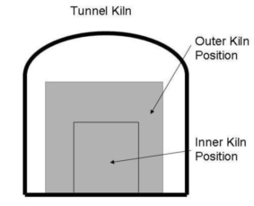
Figure 5.11 Tunnel Kiln
Unfortunately in 1950 the Ina tile company could not afford to install instrumentation to control the temperature gradient in their kiln. Therefore, Taguchi called the temperature gradient a noise factor that could not be controlled. There were other factors that could be easily controlled. Taguchi sought to find a combination of settings of these controllable factors, through use of an experimental design, that could mitigate the influence of the noise factor. This is referred to as a Robust Design Experiment. Figure 5.12 diagrammatically illustrates the factors and response for a Robust Design Experiment.
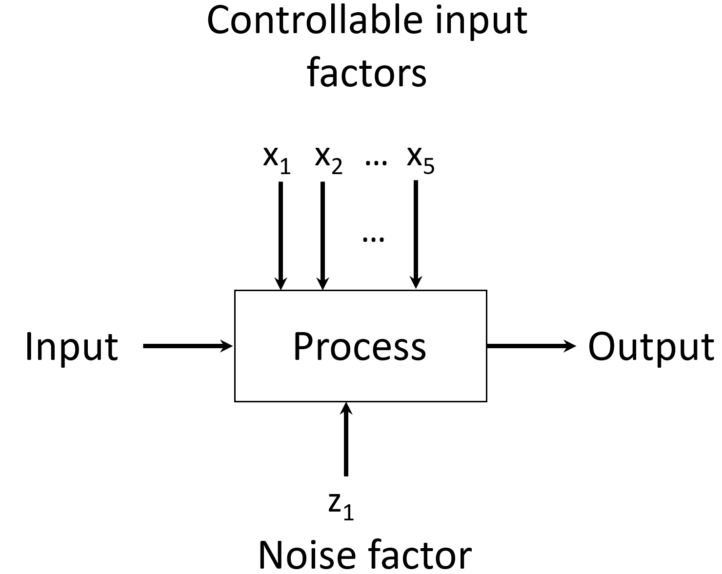
Figure 5.12 Robust Design
Figure 5.13 is a flow diagram of the process to make tiles at the Ina tile company

Figure 5.13 Tile Manufacturing Process
The variables involved in the first step in Figure 5.12 could be easily controlled. Therefore, 5 of these factors were chosen to experiment with, and the uncontrollable temperature gradient was simulated by sampling tiles from the center and outsides of the tunnel kiln, then measuring their dimensions. Table 5.7 shows the factors and levels for the Robust Design Experiment.
Table 5.7 Factors in Robust Design Experiment
| Controllable Factors | Level(\(-\)) | Level(\(+\)) |
|---|---|---|
| A–kind of agalmatolite | existing | new |
| B–fineness of additive | courser | finer |
| C–content of waste return | 0% | 4% |
| D–content of lime | 1% | 5% |
| E–content of feldspar | 0% | 5% |
| ————————– | —————- | —————- |
| Noise Factor | Level(\(-\)) | Level(\(+\)) |
| ————————– | —————- | —————- |
| F–furnace position of tile | center | outside |
A \(2^{5-1}\) fractional factorial experiment was used with the generator \(E=ABCD\). Figure 5.14 shows the list of experiments in standard order and the resulting average tile dimensions. Each experiment in the \(2^{5-1}\) design was repeated at both levels of factor F. By doing this the design changes from a \(2^{5-1}\) to a \(2^{6-1}\), and the defining relation changes from \(I=ABCDE\) to \(I=-ABCDEF\).
Table 5.8 List of Experiments and Results for Robust Design Experiment
| Random Run No. | \(A\) | \(B\) | \(C\) | \(D\) | \(E\) | \(F\)=Furnace Position | center | outside |
|---|---|---|---|---|---|---|---|---|
| 15 | \(-\) | \(-\) | \(-\) | \(-\) | \(+\) | 10.14672 | 10.14057 | |
| 13 | \(+\) | \(-\) | \(-\) | \(-\) | \(-\) | 10.18401 | 10.15061 | |
| 11 | \(-\) | \(+\) | \(-\) | \(-\) | \(-\) | 10.15383 | 10.15888 | |
| 1 | \(+\) | \(+\) | \(-\) | \(-\) | \(+\) | 10.14803 | 10.13772 | |
| 10 | \(-\) | \(-\) | \(+\) | \(-\) | \(-\) | 10.15425 | 10.15794 | |
| 2 | \(+\) | \(-\) | \(+\) | \(-\) | \(+\) | 10.16879 | 10.15545 | |
| 3 | \(-\) | \(+\) | \(+\) | \(-\) | \(+\) | 10.16728 | 10.15628 | |
| 12 | \(+\) | \(+\) | \(+\) | \(-\) | \(-\) | 10.16039 | 10.17175 | |
| 16 | \(-\) | \(-\) | \(-\) | \(+\) | \(-\) | 10.17273 | 10.12570 | |
| 8 | \(+\) | \(-\) | \(-\) | \(+\) | \(+\) | 10.16888 | 10.13028 | |
| 9 | \(-\) | \(+\) | \(-\) | \(+\) | \(+\) | 10.19741 | 10.15836 | |
| 14 | \(+\) | \(+\) | \(-\) | \(+\) | \(-\) | 10.19518 | 10.14300 | |
| 6 | \(-\) | \(-\) | \(+\) | \(+\) | \(+\) | 10.17892 | 10.13132 | |
| 5 | \(+\) | \(-\) | \(+\) | \(+\) | \(-\) | 10.16295 | 10.12587 | |
| 7 | \(-\) | \(+\) | \(+\) | \(+\) | \(-\) | 10.19351 | 10.13694 | |
| 4 | \(+\) | \(+\) | \(+\) | \(+\) | \(+\) | 10.19278 | 10.11500 |
In the R code shown below, the \(\verb!FrF2()!\) function was used to create the design in the standard order, and the vector \(\verb!y!\) contains the data. Since the design is resolution VI, all main effects and two-factor interactions can be estimated if four-factor and higher order interactions are assumed to be negligible. There are only 6 main effects and \({6 \choose 2}=15\) two-factor interactions but 32 observations. Therefore the command \(\verb!mod<-lm(y~(.)^3,data=DesF)!\) was used to fit the saturated model which includes 10 pairs of confounded or aliased three-factor interactions in addition to the main effects and two-factor interactions. The \(\verb!aliases(mod)!\) shows the alias for each three-factor interaction estimated, and the output of this command is shown below the code.
library(FrF2)
DesF<-FrF2(32,factor.names=list(A="",B="",C="",D="",F="",E=""),
           generators=list(-c(1,2,3,4,5)),randomize=FALSE)
y<-c(10.14057,10.15061,10.15888,10.13772,10.15794,10.15545,10.15628,10.17175,
     10.14672,10.18401,10.15383,10.14803,10.15425,10.16879,10.16728,10.16039,
     10.12570,10.13028,10.15836,10.14300,10.13132,10.12587,10.13694,10.11500,
     10.17273,10.16888,10.19741,10.19518,10.17892,10.16295,10.19351,10.19278)
mod<-lm(y~(.)^3,data=DesF)
aliases(mod)

A:B:C = -D:F:E
A:B:D = -C:F:E
A:B:F = -C:D:E
A:B:E = -C:D:F
A:C:D = -B:F:E
A:C:F = -B:D:E
A:C:E = -B:D:F
A:D:F = -B:C:E
A:D:E = -B:C:F
A:F:E = -B:C:D

summary(mod)
library(daewr)
fullnormal(coef(mod)[2:32],alpha=.01,refline="FALSE")
interaction.plot(Furnace_position,Content_Lime,resp)
\(\verb!fullnormal(coef(mod)[2:32],alpha=.01,refline="FALSE")!\) creates a full normal plot of the 31 estimable effects from the 32-run design. This plot is shown in Figure 5.14. It shows that the only significant effects appear to be main effect D-the content of lime and the interaction between factor D and the noise factor F-furnace position.
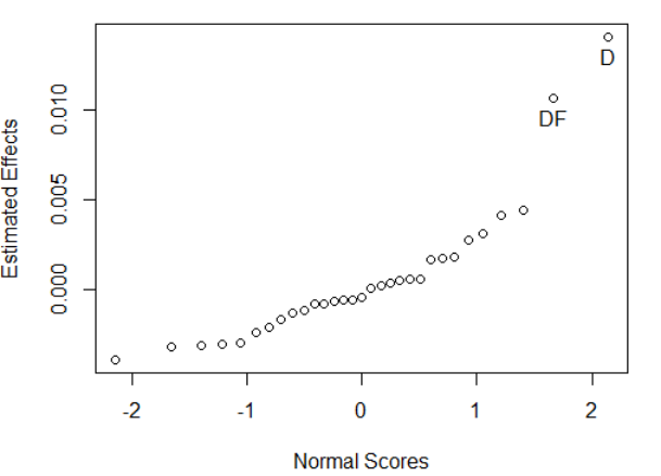
Figure 5.14 Normal Plot of Half-Effects
The \(\verb!interaction.plot(Furnace_position,Content_Lime,resp)!\) command creates the interaction plot shown in Figure 5.15 (minus the color enhancements that were added later). In this plot the noise factor is on the horizontal axis and the two lines represent the conditional main effect of F-furnace position for each level of D-content of lime. The plot shows that Furnace position effect is much stronger when there is only 1% of lime in the raw materials.
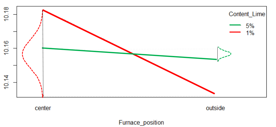
Figure 5.15 CD Interaction Plot
By adding 5% lime to the raw materials the effect of the furnace position (or temperature gradient) is greatly reduced. The red and green normal curves on the left and right of the lines representing the conditional effect of furnace position illustrate the variability in tile size expected to be caused by the uncontrollable temperature gradient. That expected variation is much less when 5% lime is added to the raw materials even though nothing was done to control the temperature gradient.
In this fractional factorial example, discovering the interaction was again key to solving the problem. In Robust Design Experiments the goal is always to find interactions between the controllable factors and the noise factors. In that way it may be possible to select a level of a control factor (or combination of levels of control factors) that reduce the influence of the noise factors and thereby decrease the variability in the response or quality characteristic of interest. In this way, the process capability index can be increased.
5.4.3 One-Quarter and Higher Order Fractions of \(2^k\) Designs
In a one-quarter fraction of a \(2^k\) design, every main effect or interaction that can be estimated will be confounded with three other effects or interactions that must be assumed to be negligible. When creating a \(\frac{1}{4}\)th fraction of a \(2^k\) design, start with a full factorial in \(k-2\) factors (i.e., the \(2^{k-2}\) base design). Next, assign the \(k-1\)st and \(k\)th factors to interactions in in the \(2^{k-2}\) base design. For example, to create a \(\frac{1}{4}\)th fraction of a \(2^5\) design start with a \(2^3\) 8-run base design. Assign the 4th factor to the \(ABC\) interaction in the base design, and the 5th factor to one of the interactions \(AB\), \(AC\), or \(BC\). If the 5th factor is assigned to \(AB\), then the defining relation for the design will be: \[\begin{equation} I=ABCD=ABE=CDE, \tag{5.8} \end{equation}\]
where \(CDE\) is found when multiplying \(ABCD\times ABE = A^2B^2CDE\)
This is a resolution III design, since the shortest word in the defining relation (other than \(I\)) has three letters. This means that some main effects will be confounded with two-factor interactions. All estimable effects will be confounded with three additional effects that must be assumed negligible. For example, main effect \(A\) will be confounded with \(BCD\), \(BE\), and \(ACDE\), which were found by multiplying all four sides of the defining relation by \(A\).
In a one-eighth fraction each main effect or or interaction that can be estimated will be confounded with 7 additional effects that must be considered negligible. When creating one-fourth or higher order fractions of a \(2^k\) factorial design, extreme care must be taken when assigning the generators or interactions in the base design to which additional factors are assigned. Otherwise, two main effects may be confounded with each other. When using the \(\verb!FrF2()!\) function to create a higher order fractional design, leave off the argument \(\verb!generators=c( )!\). The \(\verb!FrF2()!\) function has an algorithm that will produce the minimum aberration-maximum resolution design for the fraction size defined by the number of runs and number of factors. This design will have the least confounding among main effects and low order interactions that is possible.
Although, the confounding among main effects and interactions makes it seem like the analysis and interpretation of results will be complicated, the example, and additional principles presented in the next section, will clarify how this can be done.
5.4.4 An Example of a \(\frac{1}{8}\)th fraction of a \(2^7\) Design.
Large variation in the viscosity measurements of a chemical product were observed in an analytical laboratory (Snee 1985). The viscosity was a key quality characteristic of a high volume product. Since it was impossible to control viscosity without being able to measure it accurately, it was decided to conduct a ruggedness test [J. and Steiner (1975), (Wernimount 1977) of the measurement process to see which variables if any influenced the viscosity measurement. Discussions about how the measurement process worked identified 7 possible factors that could be important. A description of the measurement process and possible factors follows.
“The sample was prepared by one of two methods (M1,M2) using moisture measurements made on a volume or weight basis. The sample was then put into a machine and mixed at a given speed (800–1600 rpm) for a specified time period (0.5–3 hrs.) and allowed to”heal" for one to two hours. The levels of the variables A–E shown in Table 5.9 were those routinely used by laboratory personnel making the viscosity measurements. There were also two spindles (S1,S2) used in the mixer that were thought to be identical. The apparatus also had a protective lid for safety purposes and it was decided to run tests with and without the lid to see if it had any effect" (Snee 1985).
Table 5.9 Factors and Levels in Ruggedness Experiment
| Factors | Level (-) | Level (+) |
|---|---|---|
| A–Sample Preparation | M1 | M2 |
| B–Moisture measurement | Volume | Weight |
| C–Mixing Speed(rpm ) | 800 | 1600 |
| D–Mixing Time(hrs) | 0.5 | 3 |
| E–Healing Time(hrs) | 1 | 2 |
| F–Spindle | S1 | S2 |
| G–Protective Lid | Absent | Present |
A one-eighth fraction (\(2^{7-3}\)) was constructed with generators \(E=BCD\), \(F=ACD\), and \(G=ABC\). Samples of product from a common source were tested at the 16 conditions in the design. If the measurement process were rugged, then the differences in the measurements should have been due only to random measurement error.
To match the design in the article, the arguments \(\verb!generators=c("BCD","ACD","ABC")!\) and \(\verb!randomize=FALSE!\) were used in the call to the \(\verb!FrF2!\) function call that created the design as shown in the R code and output below.
library(FrF2)
frac1<-FrF2(16,7,generators=c("BCD","ACD","ABC"),randomize=FALSE)
frac1
    A  B  C  D  E  F  G
1  -1 -1 -1 -1 -1 -1 -1
2   1 -1 -1 -1 -1  1  1
3  -1  1 -1 -1  1 -1  1
4   1  1 -1 -1  1  1 -1
5  -1 -1  1 -1  1  1  1
6   1 -1  1 -1  1 -1 -1
7  -1  1  1 -1 -1  1 -1
8   1  1  1 -1 -1 -1  1
9  -1 -1 -1  1  1  1 -1
10  1 -1 -1  1  1 -1  1
11 -1  1 -1  1 -1  1  1
12  1  1 -1  1 -1 -1 -1
13 -1 -1  1  1 -1 -1  1
14  1 -1  1  1 -1  1 -1
15 -1  1  1  1  1 -1 -1
16  1  1  1  1  1  1  1
class=design, type= FrF2.generators
The viscosity measurements obtained after running the experiments and the Alias Pattern for the design (including only up to 4 factor interactions) is shown in the code examples below along with the calculated effects.
library(daewr)
library(FrF2)
viscosity<-c(2796,2460,2904,2320,2800,3772,2420,3376,2220,2548,2080,2464,3216,2380,
             3196,2340)
aliases(lm(viscosity~(.)^4, data=frac1))

 A = B:C:G = B:E:F = C:D:F = D:E:G
 B = A:C:G = A:E:F = C:D:E = D:F:G
 C = A:B:G = A:D:F = B:D:E = E:F:G
 D = A:C:F = A:E:G = B:C:E = B:F:G
 E = A:B:F = A:D:G = B:C:D = C:F:G
 F = A:B:E = A:C:D = B:D:G = C:E:G
 G = A:D:E = B:D:F = C:E:F = A:B:C
 A:B = A:C:D:E = A:D:F:G = B:C:D:F = B:D:E:G = C:G = E:F
 A:C = A:B:D:E = A:E:F:G = B:C:E:F = C:D:E:G = B:G = D:F
 A:D = A:B:C:E = A:B:F:G = B:C:D:G = B:D:E:F = C:F = E:G
 A:E = A:B:C:D = A:C:F:G = B:C:E:G = C:D:E:F = B:F = D:G
 A:F = A:B:D:G = A:C:E:G = B:C:F:G = D:E:F:G = B:E = C:D
 A:G = A:B:D:F = A:C:E:F = B:E:F:G = C:D:F:G = B:C = D:E
 B:D = A:B:C:F = A:B:E:G = A:C:D:G = A:D:E:F = C:E = F:G
 A:B:D = A:C:E = A:F:G = B:C:F = B:E:G = C:D:G = D:E:F


modf<-lm(viscosity~A+B+C+D+E+F+G+A:B+A:C+A:D+A:E+A:F+A:G+B:D+A:B:D,data=frac1)
summary(modf)
fullnormal(coef(modf)[-1],alpha=.15)

Coefficients:
            Estimate Std. Error t value Pr(>|t|)
(Intercept)  2705.75         NA      NA       NA
A1              1.75         NA      NA       NA
B1            -68.25         NA      NA       NA
C1            231.75         NA      NA       NA
D1           -150.25         NA      NA       NA
E1             56.75         NA      NA       NA
F1           -328.25         NA      NA       NA
G1              9.75         NA      NA       NA
A1:B1         -14.25         NA      NA       NA
A1:C1          27.75         NA      NA       NA
A1:D1        -124.25         NA      NA       NA
A1:E1         -19.25         NA      NA       NA
A1:F1          -4.25         NA      NA       NA
A1:G1         -36.25         NA      NA       NA
B1:D1          32.75         NA      NA       NA
A1:B1:D1       18.75         NA      NA       NA

Residual standard error: NaN on 0 degrees of freedom
Multiple R-squared:      1,	Adjusted R-squared:    NaN
F-statistic:   NaN on 15 and 0 DF,  p-value: NA
There are \(2^{7-3}\) effects and interactions that were estimated from this design, and each effect or interaction that can be estimated is confounded with 7 effects or interactions which must be assumed to be negligible. Due to this confounding, it would appear to be a difficult task to identify which factors and interactions actually had significant effects on the viscosity measurement. However, three principles that have been established by experience simplify the task. The first principle is the effect sparsity principle, the second is the hierarchical ordering principle (which was discussed earlier), and the third is the effect heredity principle.
The effect sparsity principle implies that when many factors are studied in a factorial design, usually only a small fraction of them will be found to be significant. Therefore, the normal probability plot of effects, shown in Figure 5.16 is a good way to identify the subset of significant effects and interaction effects.
Recall that the hierarchical ordering principle (that was defined earlier) states that main effects and low order interactions (like two-factor interactions) are more likely to be significant than higher order interactions (like 4 or 5-way interactions etc.).
The effect heredity principle states that interaction effects among factors that have insignificant main effects are rare, and that interactions involving factors that have significant main effects effects are much more likely to occur.
These three principles will be illustrated by determining which factors and interactions actually had significant effects on the viscosity measurement.
The normal plot of the half-effects in Figure 5.16 shows only 5 of the 15 calculated effects appear to be significant. They are the average main effects for C=Mixing speed, F=Spindle, D=Mixing Time, B=Moisture measurement, as well as the AD interaction (A=Sample Preparation method). Each of the main effects is confounded with four three-factor interactions, and three five-factor interactions as shown in the Alias pattern given above. The AD interaction is confounded with four four-factor interactions and two other two-factor interactions.
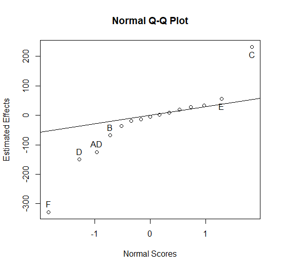
Figure 5.16 Normal Plot of Effects from Ruggedness Test
The hierarchical ordering principle leads to the belief that the main effects (rather than three or five factor interactions) caused the significance of the C, F, D, B, and E half-effects, and that a two-factor interaction rather that one of the four-factor interactions confounded with it caused the significance of AD. However, the hierarchical ordering principle does not help in determining which of the two-factor interactions AD=CF=EG caused the significance of AD.
The two largest effects (in absolute value) are C=Mixing Speed, and F=Spindle, therefore the effect heredity principle leads to the belief that the CF interaction is the cause of the confounded set of two-factor interactions AD=CF=EG.
The R code below produces the CF interaction plot shown in Figure 5.17, where it can be seen that C=Mixing speed, appears to have a larger effect on the viscosity measurement when Spindle 1 is used rather than when Spindle 2 is used.
Mixing_speed<-rep(0,16)
Spindle<-rep(1,16)
for ( i in 1:16) {
if(frac1$C[i]==-1) {Mixing_speed[i]=800} else {Mixing_speed[i]=1600}
if(frac1$F[i]==1) Spindle[i]=2
}
interaction.plot(Mixing_speed,Spindle,viscosity,type="b",pch=c(1,2),col=c(1,2))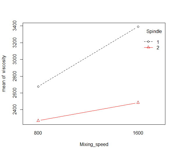
Figure 5.17 CF Interaction Plot
Additional experiments, confirmed that the CF interaction rather than AD or EG was causing the large differences in measured viscosity as seen in Figure 5.17. It was clear from the \(2^{7-3}\) experiments that the differences in measured viscosity were due to more than random measurement error. The two spindles (factor F) that were thought to be identical were not identical, and on the average viscosity measurements made using spindle 1 were 2\(\times\) 328.25=656.6 greater than viscosity measurements made using spindle 2. In addition, the difference in viscosity measurements made using spindle 1 and spindle 2 was greater when the mixing speed was 1600 rather than 800.
The results of the experimentation showed the measurement process was not rugged, and that in the future the settings for the five factors B=Moisture measurement, C=Mixing speed, D=Mixing time, E=Healing time, and F=Spindle needed to be standardized and tightly controlled in order to reduce the measurement precision.
The examples in the last two Sections of this Chapter illustrate the fact that interactions are common in experiments. Therefore full-factorial experiments like those shown in Section 5.3 or regular fractions of \(2^k\) designs like those shown in this Section (Section 5.4) are very useful in most trouble shooting or process improvement projects.
5.5 Alternative Screening Designs
In resolution III fractional factorial \(2^{k-p}\) designs some main effects will be completely confounded with two-factor interactions, and in resolution IV \(2^{k-p}\) designs some two-factor interactions will be completely confounded with other two-factor interactions. The confounding makes the analysis of these designs tricky, and follow-up experiments may be required to get independent estimates of the important main effects and two-factor interactions.
For experiments with 6, 7, or 8 factors, Alternative Screening Designs in 16 runs require no more runs than resolution III or resolution IV \(2^{k-p}\) designs. However, these designs do not have complete confounding among main effects and two-factor interactions. They have complex confounding which means that main effects are only partially confounded with two-factor interactions. Models fit to designs with complex confounding can contain some main effects and some two-factor interactions. An appropriate subset of main effects and interactions can usually be found be using forward stepwise regression.
(Hamada and Wu 1992) and (Jones and Nachtsheim 2011) suggested using a forward stepwise regression that enforces model hierarchy. In other words, when an interaction is the next term to enter the model, the parent linear main effect(s) are automatically included, if they are not already in the model. The number of steps in the forward selection procedure is the number of steps until the last term entered is still significant. When the term entered at the current step is not significant, revert to the previous step to obtain the final model. This procedure greatly simplifies the model fitting for Alternative Screening Designs.
The \(\verb!Altscreen()!\) function in the \(\verb!daewr!\) package can be used to recall 16 run Alternative Screening designs from (Jones and Montgomery 2010). The \(\verb!HierAFS()!\) function in the same package can be used to fit a model using a forward stepwise regression that enforces model hierarchy.
5.5.1 Example
(Montgomery 2005) presented an example of a 16-run 2\(_{IV}^{6-2}\) fractional factorial experiment for studying factors that affected the thickness of a photoresist layer applied to a silicon wafer in a spin coater. The factors and levels are shown in Table 5.10
Table 5.10 Factors and Levels in Spin Coater Experiment
| Factors | Level (-) | Level (+) |
|---|---|---|
| A–spin speed | \(-\) | \(+\) |
| B–acceleration | \(-\) | \(+\) |
| C–volume of resist applied | \(-\) | \(+\) |
| D–spin time | \(-\) | \(+\) |
| E–resist viscosity | \(-\) | \(+\) |
| F–exhaust rate | \(-\) | \(+\) |
In this example, the analysis showed that main effects A, B, C, and E, along with the confounded string of two-factor interactions AB=CE, were significant. However, since both main effects A and B, and main effects C and E were significant, the effect heredity principle did not help in trying to determine whether the CE interaction or the AB interaction was causing the significance of the confounded string. This is different from the last example. In that example, main effects C, F, and D were significant along with the confounded string of two-factor interaction AD=CF=EG. Since C and F were the largest main effects, the effect heredity principle would lead one to believe that CF was causing the significance of the confounded string of interactions.
Since neither the hierarchical ordering principle nor the effect heredity principle made it clear what interaction was causing the significance of the confounded string AB=CE in the present example, 16 additional follow-up experiments were run to determine which interaction was causing the significance, and to identify the optimal factor settings. The follow-up experiments were selected according to a fold-over plan (Lawson 2015), and the analysis of the combined set of 32 experiments showed that the four main effects found in the analysis of the original 16 experiments were significant along with the CE interaction.
To demonstrate the value of an Alternative Screening Design, (Johnson and Jones 2010) considered the same situation as this example. They used the model found after analysis of the combined 32 experiments, and simulated data for the photo-resist thickness. In the code below, the \(\verb!Altscreen()!\) function in the \(\verb!daewr!\) package was used to generate the same six-factor Alternative screening design used in Johnson and Jones’ article, and the thickness data was their simulated data. The \(\verb!HierAFS()!\) function identified the correct model for the simulated data in three steps, and the variable that would have entered in the fourth step, \(BE\), was not significant (p-value=0.11327). Had the original experiment been conducted with this design, no follow-up experiments would have been required, and the conclusions would have been reached with half the number of experiments.
## Registered S3 method overwritten by 'DoE.base':
##   method           from
## factorize.factor conf.designDesign<-Altscreen(nfac=6,randomize=FALSE)
Thickness<-c(4494,4592,4357,4489,4513,4483,4288,4448,4691,
4671,4219,4271,4530,4632,4337,4391)
cat("Table of Design and Response")## Table of Design and Response## A B C D E F Thickness
## 1 1 1 1 1 1 1 4494
## 2 1 1 -1 -1 -1 -1 4592
## 3 -1 -1 1 1 -1 -1 4357
## 4 -1 -1 -1 -1 1 1 4489
## 5 1 1 1 -1 1 -1 4513
## 6 1 1 -1 1 -1 1 4483
## 7 -1 -1 1 -1 -1 1 4288
## 8 -1 -1 -1 1 1 -1 4448
## 9 1 -1 1 1 1 -1 4691
## 10 1 -1 -1 -1 -1 1 4671
## 11 -1 1 1 1 -1 1 4219
## 12 -1 1 -1 -1 1 -1 4271
## 13 1 -1 1 -1 -1 -1 4530
## 14 1 -1 -1 1 1 1 4632
## 15 -1 1 1 -1 1 1 4337
## 16 -1 1 -1 1 -1 -1 4391## formula R2
## 1 y~A 0.660
## 2 y~B+A 0.791
## 3 y~C+E+C:E+B+A 0.953
## 4 y~B+E+B:E+C+C:E+A 0.965The R code below shows the calculated effects (from the \(\verb!lm()!\) function) for the model found by (Johnson and Jones 2010) and by using three steps of the \(\verb!HierAFS()!\) function. The assumptions of the least-squares fit can be checked using the \(\verb!plot.lm()!\) function as shown in the block of code above Figure 5.7.
##
## Call:
## lm(formula = Thickness ~ A + B + C + E + C:E, data = Design)
##
## Residuals:
##     Min      1Q  Median      3Q     Max
## -56.625 -19.625   2.625  23.125  53.875
##
## Coefficients:
##             Estimate Std. Error t value Pr(>|t|)
## (Intercept) 4462.875      9.494 470.073  < 2e-16 ***
## A             85.500     11.628   7.353 2.44e-05 ***
## B            -77.750     11.628  -6.687 5.45e-05 ***
## C            -34.250      9.494  -3.608  0.00479 **
## E             21.500      9.494   2.265  0.04700 *
## C:E           54.750     13.427   4.078  0.00222 **
## ---
## Signif. codes:  0 '***' 0.001 '**' 0.01 '*' 0.05 '.' 0.1 ' ' 1
##
## Residual standard error: 37.98 on 10 degrees of freedom
## Multiple R-squared:  0.9533,	Adjusted R-squared:   0.93
## F-statistic: 40.85 on 5 and 10 DF,  p-value: 2.447e-06
A=spin speed had a positive effect on thickness, and increasing spin speed increased thickness. B=acceleration had a negative effect on thickness and increasing acceleration decreased thickness. Because of the significant interaction, it is difficult to say from the main effects only what combinations of C=volume of resist applied, and E=resist viscosity would increase or decrease the thickness. The code below produces the interaction plot shown in Figure 5.18. This plot makes it clear.
interaction.plot(Design$C,resist_viscosity,Thickness,type="b",
                 xlab="volume of resist applied",
                 pch=c(1,2),col=c(1,2))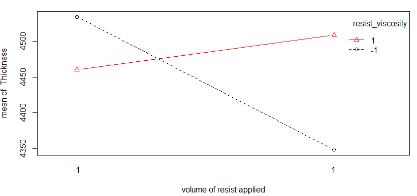
Figure 5.18 CE Interaction Plot
The greatest thickness results with a low C=volume of resist applied and a low E=resist viscosity, and the smallest thickness is produced using low E=resist viscosity but a high C=volume of resist applied.
5.6 Response Surface and Definitive Screening Experiments
The prediction model for a \(2^k\) factorial design, a \(2^{k-p}\) fractional factorial design, or an Alternative Screening design that includes the significant main effects and two-factor interactions only, would include a subset of the terms in Equation (5.9).
\[\begin{equation} y=\beta_0+\sum_{i=1}^k \beta_i X_i + \mathop{\sum^k \sum^k}_{{i<j}}\beta_{ij}X_iX_j+\epsilon, \tag{5.9} \end{equation}\]
where \(X_i\) for \(i=1 \ldots, k\) are the coded and scaled factor levels from Equation (5.2).
This equation will make accurate predictions of the response \(y\) between the high and low levels of all factors as long as the relationship between the factor levels and response \(y\) are approximately linear. If there is a curvilinear relation between the response and factor levels, a maximum, minimum or a desired target level of the response may be interior to the experimental region shown in Figure 5.20. However, the model shown in Equation (5.9), can only predict the maximum or minimum to be along the perimeter or in the corner of the experimental region.
When all the factors have quantitative levels and there is a curvilinear relation between the response and factor levels, it is necessary to fit a non-linear model like Equation (5.10) to identify the optimum process conditions.
\[\begin{equation} y=f(X_1,\ldots,X_k)+\epsilon. \tag{5.10} \end{equation}\]
This is impossible unless the form of the non-linear equation \(f(X_1,\ldots,X_k)\) is known, but using the tools of Response Surface Methodology any unknown equation can usually be well approximated by a two-term Taylor Series expansion about the center of the design region and within a limited range on the factors. The Taylor Series expansion results in a quadratic form of the equation shown in (5.11).
\[\begin{equation} y=\beta_0+\sum_{i=1}^k \beta_i X_i + \sum_{i=1}^k \beta_{ii} X_i^2+\mathop{\sum^k \sum^k}_{{i<j}}\beta_{ij}X_iX_j+\epsilon, \tag{5.11} \end{equation}\]
where again \(X_i\) for \(i=1 \ldots, k\) are the coded and scaled factor levels from Equation (5.2). Figure 5.20 is a representation of one type quadratic equation in two factors \(X_1\) and \(X_2\). In this figure it can be seen that the minimum response lies within the experimental region near the mid-level of \(X_1\) and toward the low level of \(X_2\). The model for a factorial experiment like Equation (5.1) (represented by the plane above the surface in Figure 5.19) would be incapable of predicting the location of the minimum response. For this reason the ISO Technical Committee 69 recognized the importance of Response Surface experimentation for process improvement studies, in addition to \(2^k\) factorial and \(2^{k-p}\) fractional factorial designs(Johnson and Boulanger 2012).
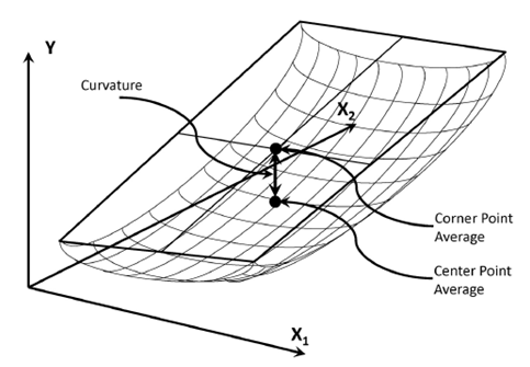
Figure 5.19 Quadratic Response Surface Model
In order to fit a quadratic equation to the data obtained from experiments, there must be at least three levels of each factor rather than the two levels contained in the \(2^k\) factorial designs, \(2^{k-p}\) fractional factorial designs, or Alternative Screening designs.
One classical experimental design used in Response Surface Methodology is the Central Composite Design. It has five levels for each factor and is composed of a \(2^k\) design, plus a center point at the center-level of each factor, plus axial or star points that are outside the \(2^k\) region. Figure 5.20 shows a visual representation of the experiments for a Central Composite Design in three factors.
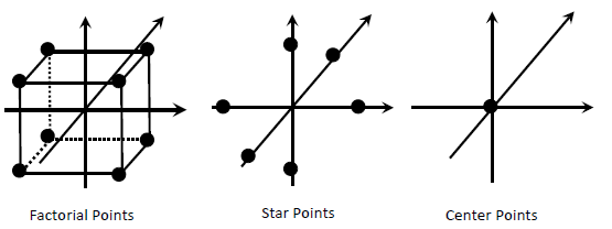
Figure 5.20 Central Composite Design
Table 5.11 is a list of the runs in a Central Composite Design in three coded and scaled factors \(X_i\), for \(i=1,\ldots,3\). In this table \(\alpha=\sqrt{3}\), and is outside the coded low-high range of \(-1\) to \(1\). In general \(\alpha=\sqrt{k}\), where \(k\) is the number of factors in the design.
Table 5.11 List of Runs for Central Composite Design in 3 Factors
| Run | \(X_1\) | \(X_2\) | \(X_3\) | |
|---|---|---|---|---|
| 1 | \(-1\) | \(-1\) | \(-1\) | Factorial |
| 2 | \(1\) | \(-1\) | \(-1\) | Points |
| 3 | \(-1\) | \(1\) | \(-1\) | |
| 4 | \(1\) | \(1\) | \(-1\) | |
| 5 | \(-1\) | \(-1\) | \(1\) | |
| 6 | \(1\) | \(-1\) | \(1\) | |
| 7 | \(-1\) | \(1\) | \(1\) | |
| 8 | \(1\) | \(1\) | \(1\) | |
| 9 | \(-\alpha\) | \(0\) | \(0\) | Axial |
| 10 | \(\alpha\) | \(0\) | \(0\) | Points |
| 11 | \(0\) | \(-\alpha\) | \(0\) | |
| 12 | \(0\) | \(\alpha\) | \(0\) | |
| 13 | \(0\) | \(0\) | \(-\alpha\) | |
| 14 | \(0\) | \(0\) | \(\alpha\) | |
| 15 | \(0\) | \(0\) | \(0\) | Center Points |
Table 5.12 shows the total number of runs or experiments required for a Central composite design that includes 5 center points. The first number \(2^k\) is the number of factorial points, the second number \(2\times k\) is the number of axial points, and the third number is the number of center points. It can be seen that even for five factors, the number of runs or experiments for a Central Composite can be excessive. One way to reduce the number of runs is to substitute a resolution V \(2^{k-p}\) design for the factorial portion, but even doing that, the number of runs required for a typical process improvement study with 7 or more factors can be impractical.
Table 5.12 Number of runs for Central Composite Design
| Number of factors \(k\) | Number of Runs |
|---|---|
| 2 | \(2^2\)+4+5=13 |
| 3 | \(2^3\)+6+5=19 |
| 4 | \(2^4\)+8+5=29 |
| 5 | \(2^5\)+10+5=47 |
| 6 | \(2^6\)+12+5=81 |
| 7 | \(2^7\)+14+5=157 |
In order to reduce the number of runs required, the traditional approach is to experiment sequentially. Start with a resolution III or IV \(2^{k-p}\) design, and identify which factors are significant. Next, augment the design with follow-up experiments to obtain unconfounded estimates of the significant main effects and two-factor interactions. Finally, add center points and axial points for the significant effects, in order to fit a subset of the terms in Equation (5.11). Figure 5.21 outlines this strategy.
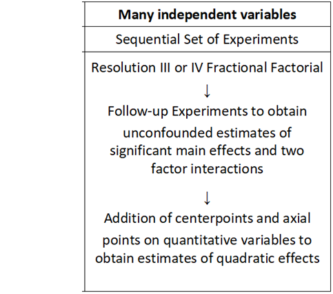
Figure 5.21 Sequential Experimentation Strategy
In 2011, Jones and Nachtsheim proposed the use of Definitive Screening Designs that reduce the number of experiments required to fit a subset of Equation (5.11) in the significant factors. Their approach essentially combines an efficient screening design, for identifying important factors and interactions, with center levels for the factors that allow fitting quadratic effects. These designs can be called super-saturated in that the number of runs in the design (\(2\times k+1\)) is less than the number of coefficients \(\left(1 + 2\times k + \frac{k\times (k-1)}{2}\right)\) in Equation (5.11).
However, if there are several proposed factors in a process improvement study, it is unlikely that each factor will have significant linear, quadratic, and interaction terms with all the other factors. This is again because of the effect sparsity principle. When using a Definitive Screening design, like an Alternative Screening design, an appropriate model consisting of the important subset of terms in Equation (5.11) can usually be obtained using a forward selection procedure.
When using a Definitive Screening Design, the selection procedure should take into account the special structure of the design (Jones and Nachtsheim 2017). The special structure of Definitive Screening designs is that all linear main effects are completely unconfounded with all quadratic and two-factor interaction terms. Quadratic and two-factor interaction terms are partially confounded like they are in Alternative Screening Designs. Therefore, when using a Definitive Screening design, the important main effects can be determined first, and then, assuming strong effect heredity, a forward search is made with candidates being the quadratic terms and two-factor interactions involving the important main effects.
Jones and Nachtsheim’s 2011 paper listed a catalog of Definitive Screening Designs. The \(\verb!DefScreen()!\) function in the R package \(\verb!daewr!\) can be used to recall a design from this catalog. The example below illustrates this.
##     A  B  C  D  E  F  G  H
## 1   0 -1  1  1 -1  1  1  1
## 2   0  1 -1 -1  1 -1 -1 -1
## 3  -1  0 -1  1  1  1  1 -1
## 4   1  0  1 -1 -1 -1 -1  1
## 5  -1 -1  0  1  1 -1 -1  1
## 6   1  1  0 -1 -1  1  1 -1
## 7   1 -1  1  0  1  1 -1 -1
## 8  -1  1 -1  0 -1 -1  1  1
## 9  -1 -1  1 -1  0 -1  1 -1
## 10  1  1 -1  1  0  1 -1  1
## 11  1 -1 -1 -1  1  0  1  1
## 12 -1  1  1  1 -1  0 -1 -1
## 13 -1  1  1 -1  1  1  0  1
## 14  1 -1 -1  1 -1 -1  0 -1
## 15  1  1  1  1  1 -1  1  0
## 16 -1 -1 -1 -1 -1  1 -1  0
## 17  0  0  0  0  0  0  0  0
The argument \(\verb!m=8!\) specifies that there are 8 quantitative 3-level factors in the design. The number of runs is \(2\times k+1=17\), when \(k=8\). This design is listed in standard order since the default option \(\verb!randomize=FALSE!\) was not overridden in the function call. When planning a Definitive Screening design, the option \(\verb!randomize=TRUE!\) should be used to recall the runs in a random order, and thus prevent biases from changes in unknown factors.
To illustrate the analysis of data from an Definitive Screening design, consider the following example. (Libbrecht et al. 2015) completed an 11-run Definitive Screening Design for optimizing the process of synthesizing soft template mesoporus carbons. Mesoporus carbons can be used for various applications such as electrode materials, absorbents, gas storage hosts, and support material for catalysts. The effect of five synthesis factors on the material properties of the carbons were considered. Because the relationship between the material properties, or responses, and the synthesis parameters, or factors, was expected to be nonlinear it was desirable to use an experimental design that would allow fitting a subset of the terms in Equation 5.11. The five factors studied were: A (Carbonation temperature [°C]), B (Ratio of precursor/surfactant), C (EISA-Time [h]), D (Curing time [h]), and E (EISA surface area [cm\(^2\)]). Table 5.13 shows the range of each of the five factors.
Table 5.13 Factors and Uncoded Low and High Levels in Mesoporus Carbon Experiment
| Factors | Level (-) | Level (+) |
|---|---|---|
| A–Carbonation temperature | 600(°C) | 1000(°C) |
| B–Ratio of precursor to surfactant | 0.7 | 1.3 |
| C–EISA-Time | 6 h | 24 h |
| D–Curing time | 12 h | 24 h |
| E–EISA surface area | 65(cm\(^2\)) | 306(cm\(^2\)) |
The experimental outputs or properties of the mesoporus carbon were microporus and mesoporus surface area and pore volumes and the weight % carbon. Among the purposes of the experimentation was to understand the effects of the acid catalyzed EISA synthesis parameters on the material properties, and to find the optimal set of synthesis parameters to maximize mesopore surface area.
A traditional central composite design for five factors would entail 47 experiments. Since it was doubtful that all terms in a Equation 5.11 for \(k=\) five factors would be significant, a Definitive Screening Design using less than one fourth that number of experiments (11) could be used.
The R code below shows the command to create the Definitive Screening Design using the \(\verb!DefScreen()!\) function. The \(\verb!randomize=FALSE!\) option was used for this experiment to create the design in standard order. The actual experiments were conducted in random order, but by creating the design in standard order, it was easier to pair the responses shown in the article to the experimental runs. The factor levels are in coded and scaled units. All Definitive Screening designs in Jones and Nachtsheim’s catalog as recalled by the \(\verb!DefScreen!\) function contain one center point where all factors are set at their mid levels. In This experiment, there were three center points. Including additional centerpoints allows for a lack of fit test to be performed. The argument \(\verb!center=2!\) tells the function to add two additional center points.
##     A  B  C  D  E
## 1   0  1  1 -1 -1
## 2   0 -1 -1  1  1
## 3   1  0 -1 -1  1
## 4  -1  0  1  1 -1
## 5   1 -1  0  1 -1
## 6  -1  1  0 -1  1
## 7   1 -1  1  0  1
## 8  -1  1 -1  0 -1
## 9   1  1  1  1  0
## 10 -1 -1 -1 -1  0
## 11  0  0  0  0  0
## 12  0  0  0  0  0
## 13  0  0  0  0  0
In the design listing shown above, the three center points (runs 11, 12, and 13) can be seen to have the center level (in coded and scaled units) for each factor.
The code below shows the responses recorded from the synthesis experiments, and the call of the function \(\verb!FitDefSc()!\) used to fit a model to the data. The response, \(\verb!Smeso!\), is the mesoporus surface area. The option \(\verb!alpha=.05!\) controls the number of second order terms that will be allowed in the model. A smaller the value of \(\verb!alpha!\) is more stringent and allows fewer second order terms to enter. A larger value of \(\verb!alpha!\) is less stringent and allows more second order terms to enter. Using the \(\verb!FitDefSc()!\) values of \(\verb!alpha=.05!\) within the range .05 - .20 should be used.
library(daewr)
Smeso<-c(241,295,260,338,320,265,275,248,92.5,383,313,305,304)
FitDefSc(Smeso,design,alpha=.05)
##
## Call:
## lm(formula = y ~ (.), data = ndesign)
##
## Residuals:
## Min 1Q Median 3Q Max
## -13.667 -3.653 0.000 3.550 12.373
##
## Coefficients:
## Estimate Std. Error t value Pr(>|t|)
## (Intercept) 304.000 5.012 60.656 1.35e-09 ***
## B -76.030 4.362 -17.429 2.29e-06 ***
## D -26.609 4.533 -5.870 0.001082 **
## B:D -21.023 4.779 -4.399 0.004572 **
## I(B^2) -44.318 6.500 -6.819 0.000488 ***
## A -42.803 4.362 -9.812 6.45e-05 ***
## E -21.459 4.533 -4.734 0.003213 **
## ---
## Signif. codes: 0 '***' 0.001 '**' 0.01 '*' 0.05 '.' 0.1 ' ' 1
##
## Residual standard error: 11.21 on 6 degrees of freedom
## Multiple R-squared: 0.9866, Adjusted R-squared: 0.9733
## F-statistic: 73.9 on 6 and 6 DF, p-value: 2.333e-05
##
## Sums of Squares df F-value P-value
## Lack of Fit 704.89318 4 7.24205 0.04059
## Pure Error 48.66667 2The lack of fit F-test shown at the bottom of the output is only produced when there is more than one center point in the design. The F-ratio compares the variability among the replicated center point responses, and the lack of fit variability, or variability among the residuals (i.e., actual responses\(-\)fitted values) minus the variability among replicate center points. In this example, the F-test is significant. This means the difference in predictions from the fitted model and new experiments at the prediction conditions will be larger than replicate experiments at those conditions.
To improve the model, \(\verb!alpha!\) was increased as shown in the code below to expand the model.
##
## Call:
## lm(formula = y ~ (.), data = ndesign)
##
## Residuals:
##        1        2        3        4        5        6        7        8
## -0.39670 -2.32094  0.46480  3.15873 -0.12433  1.03021  3.54358  0.07995
##        9       10       11       12       13
## -0.71346 -1.09831  4.45882 -3.54118 -4.54118
##
## Coefficients:
##             Estimate Std. Error t value Pr(>|t|)
## (Intercept)  308.541      2.386 129.329 2.14e-08 ***
## I(D^2)       -11.353      3.046  -3.727 0.020353 *
## D            -26.609      1.855 -14.343 0.000137 ***
## B            -76.030      1.785 -42.589 1.82e-06 ***
## E            -21.459      1.855 -11.567 0.000319 ***
## B:E           11.344      2.125   5.338 0.005933 **
## B:D          -21.024      1.974 -10.649 0.000440 ***
## I(B^2)       -37.509      2.974 -12.611 0.000228 ***
## A            -42.803      1.785 -23.976 1.79e-05 ***
## ---
## Signif. codes:  0 '***' 0.001 '**' 0.01 '*' 0.05 '.' 0.1 ' ' 1
##
## Residual standard error: 4.586 on 4 degrees of freedom
## Multiple R-squared:  0.9985,	Adjusted R-squared:  0.9955
## F-statistic: 334.9 on 8 and 4 DF,  p-value: 2.216e-05
##
##             Sums of Squares  df F-value P-value
## Lack of Fit        35.46992   2 0.72883 0.57842
## Pure Error         48.66667   2
In the output it can be seen that two additional terms (\(\verb!(I(D^2)!\), and \(\verb! B:E)!\)) were added to the model and the lack of fit test is no longer significant. This means that predictions from this fitted model will be just as accurate as running additional experiments at the factor levels where the predictions are made.
Sometimes the \(\verb!FitDefSc()!\) may include some terms in the model that are not significant at the \(\alpha=.05\) level of significance. If that is the case, the \(\verb!lm()!\) function can be used, as shown in the example in Section 5.5.1, to refit the model eliminating the insignificant term with the largest p-value. This can be repeated until all remaining terms in the model are significant. After using the \(\verb!lm()!\) function to fit a model, the assumptions of the least-squares fit can be checked by looking at the diagnostic plots produced by the \(\verb!plot.lm()!\) functions as shown in the block of R code before Figure 5.7
Predictions from the fitted model can be explored graphically to identify the optimal set of synthesis parameters to maximize mesopore surface area, \(\verb!Smeso!\). Figure 5.22 shows contour plots of the predicted mesoporus surface area as a function of curing time and ratio of precursor/surfactant. The plot on the left is made when EISA surface area is at its low level of 65, and the plot on right is when EISA surface area is at its high level of 306. The code for producing these plots is in the R code for Chapter 5.
Figure 5.22 Contour Plots of Fitted Surface
It can be seen that the maximum predicted mesopore surface area is just over 400(m\(^2\)/g) when carbonation temperature \(=\) 600, Ratio \(\approx\) .80, EISA time \(=\) 15, curing time \(\approx\) 15, and EISA surface area \(=\) 65. These conclusions were reached after conducting only 13 experiments, far less than would be required using the traditional approach illustrated in Figure 5.21. The R function \(\verb!ConstrOptim()!\) can also be used to get the optimal combination synthesis parameters numerically. For an example see (Lawson 2015).
5.7 Summary
This chapter has illustrated \(2^k\) factorial designs and \(2^{k-p}\) fractional factorial designs and Alternative Screening designs for estimating main effects and interactions and identifying the important subset of terms in Equation 5.9. These designs are useful for identifying optimal processing conditions on a boundary or corner of the experimental region. Definitive Screening Designs were introduced as an efficient way of finding the important subset of terms in Equation 5.11, and for identifying optimal process conditions within the experimental region. There are many additional and useful experimental designs for estimating main effects, interaction effects, and non-linear effects with multiple factors.
5.8 Additional Reading
Plackett-Burman designs(Plackett and Burman 1946) and Model-Robust designs(Li and Nachtsheim 2000) are additional designs that have a minimal number of runs and complex confounding among two-level factor main effects and two-factor interactions. They are similar to Alternative screening designs. They are also useful for identifying the important subset of terms in Equation 5.9 with fewer runs than traditional \(2^k\) factorial designs. (Jones and Nachtsheim 2013)) also developed a catalog of Definitive Screening designs that contain three-level quantitative factors and up to 4 additional two-level categorical factors.
Blocked designs should be used to get more precise tests of main effects and interactions when there are uncontrollable conditions that cause extra variability in experimental units. Blocked designs group similar experimental units into more homogeneous blocks to reduce the variance within the blocks. When it is very difficult or expensive to completely randomize the order of experimentation due to one or more factors with hard to change levels, split-plot designs can be used. Split plot designs are available in situations where \(2^k\) and \(2^{k-p}\) would be used if there were no factors with hard to change levels. The book by (Lawson 2015) also includes examples of R code to create and analyze data resulting from the designs just mentioned and many other useful Experimental Designs for troubleshooting and process improvement.
5.9 Exercises
Run all the code examples in the chapter as you read.
(Johnson and McNeilly 2011) describe the use of a factorial experiment to quantify the impact of process inputs on outputs so that they can meet the customer specifications. The experiments were conducted at Metalor Technologies to understand its silver powder production process. High-purity silver powder is used in conductive pastes by the microelectronics industry. Physical properties of the powder (density and surface area in particular) are critical to its performance. The experiments set out to discover how three key input variables: (1) reaction temperature, (2) %ammonium, and (3) stir rate effect the density and surface area. The results of their experiments (in standard order) are shown in the following Tables. Two replicates were run at each of the eight treatment combinations in random order.
| Factor | Level (-) | Level (+) |
|---|---|---|
| A=Ammonium | 2% | 30% |
| B=Stir Rate | 100 rpm | 150 rpm |
| C=Temperature | 8°C | 40°C |
| \(X_A\) | \(X_B\) | \(X_C\) | Density | Surface Area |
|---|---|---|---|---|
| \(-\) | \(-\) | \(-\) | 14.68, 15.18 | .40, .43 |
| \(+\) | \(-\) | \(-\) | 15.12, 17.48 | .42, .41 |
| \(-\) | \(+\) | \(-\) | 7.54, 6.66 | .69, .67 |
| \(+\) | \(+\) | \(-\) | 12.46, 12.62 | .52, .36 |
| \(-\) | \(-\) | \(+\) | 10.95, 17.68 | .58, .43 |
| \(+\) | \(-\) | \(+\) | 12.65, 15.96 | .57, .54 |
| \(-\) | \(+\) | \(+\) | 8.03, 8.84 | .68, .75 |
| \(+\) | \(+\) | \(+\) | 14.96, 14.96 | .41, .41 |
Analyze the density response. Draw conclusions about the effects of the factors. Are there any significant interactions?
Is the fitted model adequate?
Make any plots that help you explain and interpret the results.
Analyze the surface area response. Draw conclusions about the effects of the factors. Are there any significant interactions?
Is the fitted model adequate?
Make any plots that help you explain and interpret the results.
If the specifications require surface area to be between 0.3 and 0.6 cm2/g and density, must be less than 14 g/cm3, find operating conditions in terms of 1) reaction temperature, 2) % ammonium, and 3) stir rate that will result in a product that meets these specs.
Create the minimum aberration maximum resolution (\(2^{5-2}\)) design.
Create a (\(2^{5-2}\)) design using the generators D=ABC, E=AC.
What is the defining relation for this design?
what is the Alias Pattern for this design?
Not knowing what factors will be represented by A-D, can you say whether the design you created in this exercise is any better or worse than the minimum aberration maximum resolution design you created in exercise 2?
- (Hill and Demier 1970) showed an example of the use of the (\(2^{5-2}\)) design you created in exercise 3 for improving the Yield of dyestuffs to make the product economically competitive. The product formation was thought to take place by the reaction steps shown.
Figure 5.24
Where F is the basic starting material that reacts in the presence of a solvent with material C to give intermediates and then the final product. The second reaction is a condensation step, and the third reaction is a ring-closing step. It wasn’t certain what the role of materials B and E played in reactions 2 and 3. Even though there were at least these three separate reactions, preliminary laboratory runs indicated that the reactants could be charged all at once. Therefore, the reaction procedure was to run for t1 hr at T1 °C, corresponding to the steps needed for condensation, and then the temperature raised to T2 °C for t2 more hours to complete the ring-closure. Preliminary experiments indicated that the time and temperature of the condensation deserved additional study, because this step appeared more critical and less robust than the ring-closing step. Other variables thought to affect the reaction were the amount of B, E, and the solvent. Therefore, these five variables were studied in an initial screening design to determine which had significant effects on product yield. The factors and levels were:
| Factor | Level (-) | Level (+) |
|---|---|---|
| A=Condensation temp. | 90°C | 110°C |
| B=Amount of B | 29.3 cc | 39.1 cc |
| C=Solvent volume | 125 cc | 175 cc |
| D=Condensation time | 16 h | 24 h |
| E=Amount of E | 29 cc | 43 cc |
- Given that the observed Yields and Filtration times for the (\(2^{5-2}\)) experiment (in standard order) were:
Yields = 23.2,16.9,16.8,15.5,23.8,23.4,16.2,18
Filtration Time = 32,20,25,21,30,8,17,28
determine what factors and or interactions had significant effects on these responses, and interpret or explain them.
- The researchers believed that factor D=Condensation Temperature would have a large effect on both Yield and Filtration Time. The fact that it did not in these experiments, led them to believe that it may have a quadratic effect that was missed in the two-level experiments. What additional experiments would you recommend to check the possibility of a quadratic effect?
Compare the following two designs for studying the main effects and two-factor interactions among 6 factors. A=the minimum aberration maximum resolution \(2^{6-1}\) and B=an Alternative Screening design for 6 factors. Create a two-by-two table with column headings for design A. and design B., and row headings Advantages and Disadvantages. Make entries in the four cells of the table showing the advantages and disadvantages for using each of the two designs for stated the purpose.
Compare the following two designs for studing the main effects and two-factor interactions among 7 factors. A=the minimum aberration maximum resolution \(2^{7-3}\) and B=an Alternative Screening design for 7 factors. Create a two-by-two table with column headings for design A. and design B., and row headings Advantages and Disadvantages. Make entries in the four cells of the table showing the advantages and disadvantages for using each of the two designs for stated the purpose.
Which of the two designs would you recommend for the comparisom in question 6.?
Which of the two designs would you recommend for the comparisom in question 7.?
- Create a Definitive Screening design for 6 three-level main effects that includes 3 additional center points.
Create the design in standardized and randomized order.
Assumming experiments had been conducted using the design you created in (a) and the responses in standard order were: 10.95,7.83,11.26,11.31,9.81,19.94,16.33,4.90,17.36,14.57,27.30,5.65,9.27,9.30,8.77,11.11, use the \(\verb!FitDefSc()!\) function to find a model for the data.
Does the model fit the data well? (i.e., is there any significant lack of fit?)
If there are insignificant terms in the model you found, refit the model using the \(\verb!lm()!\) eliminating one term at a time until all remaining terms are significant.
Make the diagnostic plots to check the least-squares model assumptions for your final model.
References
Box, G. E. P. 1966. “Use and Abuse of Regression.” Technometrics 8 (4): 625–29.
Box, G. E. P., S. Bisgaard, and C. Fung. 1988. “An Explanation and Critique of Taguchi’s Contributions to Quality Engineering.” Quality and Reliability Engineering International 4 (2): 121–31.
Britz, G. C., D. W. Emerling, L. B. Hare, R. W. Hoerl, S. J. Janis, and J. E. Shade. 2000. Improving Performance Through Statistical Thinking. Milwaukee, Wisconsin: ASQ Quality Press.
Burke, S. E., and R. T. Silvestrini. 2017. The Certified Quality Engineer Handbook 4th Ed. Milwaukee, Wisconsin: ASQ Quality Press.
Durakovic, B. 2017. “Design of Experiments Application, Concepts, Examples: State of the Art.” Periodicicals of Engineering and Natural Sciences 5 (3): 421–39.
Hamada, M., and C. F. J Wu. 1992. “Analysis of Experiments with Complex Aliasing.” Journal of Quality Technology 24: 130–37.
Hill, W. J., and W. R. Demier. 1970. “More on Planning Experiments to Increase Research Efficiency.” Industrial and Engineering Chemistry 62 (10).
J., Youden W., and E. H. Steiner. 1975. Statistical Manual of the Association of Official Analytical Chemists. Association of Official Analytical Chemists.
Johnson, L., and K. McNeilly. 2011. “Results May Not Vary.” Quality Progress 44 (5): 61–65.
Johnson, Mark, and Bradley Jones. 2010. “Classical Design Structure of Orthogonal Designs with Six to Eight Factors and Sixteen Runs.” Quality and Reliability Engineering International 27: 61–70.
Johnson, M. E., and M. Boulanger. 2012. “Statistical Standards and ISO, Part 4 Applications Related to the Implementation of Six Sigma.” Quality Engineering 24: 552–57.
Jones, B., and D. C. Montgomery. 2010. “Alternatives to Resolution IV Screening Designs in 16 Runs.” Int. J. Experimental Design and Process Optimisation 1: 285–95.
Jones, B., and C. J. Nachtsheim. 2011. “A Class of Three-Level Designs for Definitive Screening in the Presence of Second-Order Effects.” Journal of Quality Technology 43: 1–15.
Jones, B., and C. J. Nachtsheim. 2011. “A Class of Three-Level Designs for Definitive Screening in the Presence of Second-Order Effects.” Journal of Quality Technology 43: 1–15.
2013. “Definitive Screening Designs with Added Two-Level Categorical Factors.” Journal of Quality Technology 45: 121–29.Jones, B., and C. J. Nachtsheim. 2011. “A Class of Three-Level Designs for Definitive Screening in the Presence of Second-Order Effects.” Journal of Quality Technology 43: 1–15.
2013. “Definitive Screening Designs with Added Two-Level Categorical Factors.” Journal of Quality Technology 45: 121–29. 2017. “Effective Design-Based Model Selection for Definitive Screening Designs.” Technometrics 59 (3): 319–29.Lawson, J. 2015. Design and Analysis of Experiments with R. Boca Raton, Florida: Chapman; Hall/CRC.
Li, W., and C. Nachtsheim. 2000. “Model Robust Factorial Designs.” Technometrics 42: 345–52.
Libbrecht, W., F. Deruyck, H. Poelman, A. Verberckmoes, J. Thybaut, J. DeClercq, and P. VanDerVoort. 2015. “Optimization of Soft Templated Mesoporus Carbon Cynthesis Using Definitive Screening Design.” Chemical Engineering Journal 259: 126–34.
Montgomery, D. C. 2005. Design and Analysis of Experiments. 6th ed. Hoboken, New Jersey: John Wiley & Sons.
Ott, E. R. 1975. Process Quality Control-Troubleshooting and Interpretation of Data. New York, N. Y.: McGraw-Hill.
Plackett, R. L., and J. P. Burman. 1946. “The Design of Optimum Multifactor Experiments.” Biometrika 33: 305–25.
Snee, R. D. 1985. “Experimenting with a Large Number of Variables.” In Experiments in Industry Design Analysis and Interpretation of Results, edited by Ronald Snee, Lynne B. Hare, and J. Richard Trout. Milwaukee, Wisconsin: American Society for Quality Control.
Taguchi, G., and Y. Wu. 1979. Introduction to Off-Line Quality Control. Central Japan Quality Control Association.
Wernimount, G. 1977. “Ruggedness Evaluation of Test Procedures.” ASTM Standardization News, 5: 261.