Chapter 3 : Random Slopes, Wald Tests, a Re-examination of Inference
3.1 Random Slopes
- A very common extension of multi-level models involves what are usually called random slopes.
- Up to this point, all effects were some form of random intercept, or level shift.
- You can see this by regrouping terms into a random coefficients formulation:
\[
MATHGAIN_{ijk} = (b_0 + \eta_{jk} + \zeta_k) + b_1 SES_{ijk} + b_2 MATHKNOW_{jk} + \varepsilon_{ijk}
\]
\[
\varepsilon_{ijk}\sim N(0,\sigma_\varepsilon ^2),\ \eta_{jk}\sim N(0,\sigma_\eta ^2),\ \zeta_k\sim N(0,\sigma_\zeta ^2)\mbox{ indep.}
\]
- All of the components of the first term, in parentheses, generate a school- and classroom-specific shift up or down from the mean.
- We could even re-express the equation in a form that made this explicit: \[ MATHGAIN_{ijk} = \beta_{0jk} + b_1 SES_{ijk} + b_2 MATHKNOW_{jk} + \varepsilon_{ijk}, \] where \({\beta_{0jk}} = {b_0} + {\eta_{jk}} + {\zeta_k}\) varies by both school and classroom (we sometimes call this the level 2 equation).
- It is only a small step, then, to imagine a situation in which there was variation at the group level, in the response to a predictor. E.g., the regression coefficient or effect for SES could be different depending on the school.
i. This could be important for documenting variation in policy: a school in which the effect of SES was positive (on math scores) is different from another school in which the effect of SES was negative.- Note: even if the ‘fixed effect’ for SES is non-significant, there could be significant variation in the return to SES across grouping factors (e.g., schools)4.
- Some researchers like to conceptualize random slopes as interactions between group and predictor. They are, but we do not estimate every interaction, only their distribution.
- Do we have any evidence of this in our school data?
- We first take a graphical approach to variation in coefficients – compute ‘mini regressions,’ so that slopes may vary by school (this is like including all interactions). We’ll now look at MATHGAIN vs. SES, in the first 12 schools):
Code
## `geom_smooth()` using formula = 'y ~ x'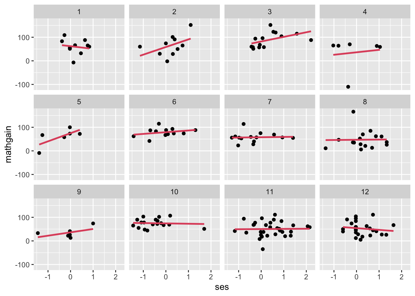
- (cont.)
- (cont.)
- We see a little variation in the slopes.
- We don’t have a good way to assess the ‘significance’ of that variation, graphically. We are building up to this ability.
- Note: This graphic is NOT helping us to fully assess the larger question, which is, “net of the fixed effects for SES & MATHKNOW and the random effects for schools and classrooms, is there remaining variation in the ‘return’ to (effect of; response surface for) SES?”
- We address that question here (by including SES and MATHKNOW in our model).
- We use an estimate of within-group residual error that we have not described yet (we will soon), but for now, accept it as a residual that can ‘net out’ the fixed and random (group) effects.
- The formula for this type of residual may be helpful to see (“hats” indicate estimates):
- (cont.)
\[ \hat{\varepsilon}_{ijk} = MATHGAIN_{ijk} - \{(\hat{b}_0 + \hat\eta_{jk} + \hat \zeta_k) + \hat b_1 SES_{ijk} + \hat b_2 MATHKNOW_{jk}\}, \]
Code
#look at residuals:
fit1 <- lmer(mathgain~ses+mathknow+(1|schoolid/classid),data=dat)
#get the right sample:
save.options <- options()
options(na.action='na.pass')
mm <- model.matrix(~mathgain+ses+mathknow,data=dat)
options(save.options)
in_sample <- apply(is.na(mm),1,sum)==0
dat$res1 <- rep(NA,dim(dat)[1]) #fill with correct number of missings
dat$res1[in_sample] <- residuals(fit1)

ggplot(data=subset(dat,schoolid<13),aes(y=res1,x=ses))+
  geom_point()+
  facet_wrap(~schoolid,nrow = 3)+
  geom_smooth(method = "lm", se = FALSE,col=2)
## `geom_smooth()` using formula = 'y ~ x'## Warning: Removed 24 rows containing non-finite values (`stat_smooth()`).## Warning: Removed 24 rows containing missing values (`geom_point()`).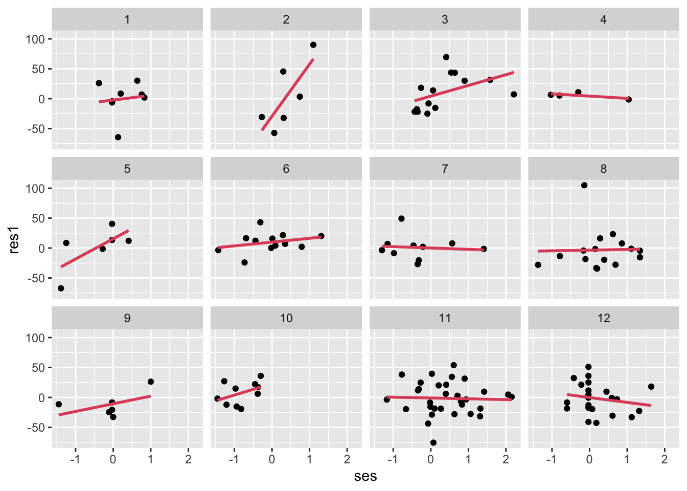
- (cont.)
- (cont.)
- Each facet (small plot) is a school; there should be no remaining relationship to SES in these residuals, right? But based on the residuals, there are likely some differences in SES slope, by school.
- We do the same comparison of residuals vs. MATHKNOW:
- (cont.)
Code
## `geom_smooth()` using formula = 'y ~ x'## Warning: Removed 24 rows containing non-finite values (`stat_smooth()`).## Warning: Removed 24 rows containing missing values (`geom_point()`).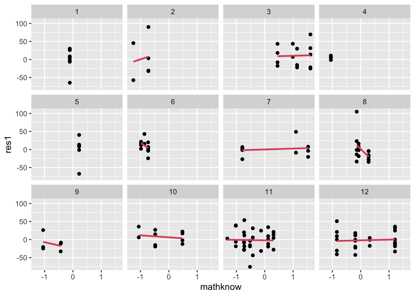
- (cont.)
- (cont.)
- There is some variation in MATHKNOW slope, as assessed using residuals, but the slopes are missing in many schools.
- Here, we face a different problem of little variation in MATHKNOW. This occurs whenever there are only a few classrooms in a school (or when all teachers in the school have the same MATHKNOW). Can you identify which schools have only one classroom sampled in this graphic (hint: can’t fit a regression line)?
- (cont.)
- One way to include variation in the returns to a predictor formally in a model uses the random coefficients formulation:
- We’ll do this first for variation in returns to SES at the school level:
\[ MATHGAIN_{ijk} = \beta_{0jk} + \beta_{1k}SES_{ijk} + b_2 MATHKNOW_{jk} + \varepsilon_{ijk} \]
\[ \beta_{0jk} = b_0 + \eta_{0jk} + \zeta_{0k},\ \beta_{1k} = b_1 + \zeta_{1k} \]
\[ \varepsilon_{ijk}\sim N(0,\sigma_\varepsilon ^2),\ \eta_{0jk}\sim N(0,\sigma_{\eta_0}^2),\ \zeta_{0k}\sim N(0,\sigma_{\zeta_0}^2),\ \zeta_{1k}\sim N(0,\sigma_{\zeta_1}^2)\mbox{ indep.} \]
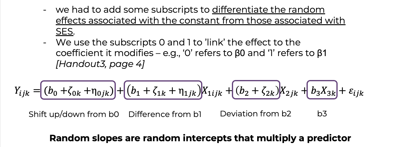
i (cont.). 1. Note that we had to add some subscripts to differentiate the random effects associated with the constant from those associated with SES. 2. Note as well that this notation is a bit harder to extend. For example, how would we add classroom-level random slopes for SES? ii. If the ‘returns’ to SES vary by classroom (j) within school (k), we need to change the index on the beta coefficient in front of SES to use the index ’jk’:
\[ MATHGAIN_{ijk} = \beta_{0jk} + \beta_{1jk}SES_{ijk} + b_2 MATHKNOW_{jk} + \varepsilon_{ijk}, \]
\[ \mbox{ with }\beta_{0jk} = b_0 + \eta_{0jk} + \zeta_{0k};\ \beta_{1jk} = b_1 + \eta_{1jk} + \zeta_{1k} \]
\[ \varepsilon_{ijk}\sim N(0,\sigma_\varepsilon ^2),\ \eta_{0jk}\sim N(0,\sigma_{\eta_0}^2),\ \eta_{1jk}\sim N(0,\sigma_{\eta_1}^2),\ \zeta_{0k}\sim N(0,\sigma_{\zeta_0}^2),\ \zeta_{1jk}\sim N(0,\sigma_{\zeta_1}^2) \mbox{ indep.} \]
ii (cont.). 2. We use the subscripts 0 and 1 to ‘link’ the effect to the coefficient it modifies – e.g., ‘0’ refers to \(\beta_0\) and ‘1’ refers to \(\beta_1\). iii. To see how the return to the predictor varies, it is useful to rearrange the components of the random coefficients in different ways. 1. For our last example:
\[ MATHGAIN_{ijk} = \beta_{0jk} + \beta_{1jk}SES_{ijk} + b_2 MATHKNOW_{jk} + \varepsilon_{ijk}, \]
\[ \mbox{with }\beta_{0jk} = b_0 + \eta_{0jk} + \zeta_{0k};\ \beta_{1jk} = b_1 + \eta_{1jk} + \zeta_{1k} \]
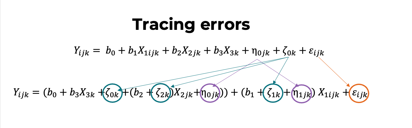
- This could also be written:
\[ MATHGAIN_{ijk} = (b_0 + \eta_{0jk} + \zeta_{0k}) + (b_1 + \eta_{1jk} + \zeta_{1k})SES_{ijk} + b_2 MATHKNOW_{jk} + \varepsilon_{ijk} \]
- It is often useful to separate out the fixed and random effects:
\[ MATHGAIN_{ijk} = b_0 + b_1 SES_{ijk} + b_2 MATHKNOW_{jk} + \eta_{0jk} + \eta_{1jk}SES_{ijk} + \zeta_{0k} + \zeta_{1k}SES_{ijk} + \varepsilon_{ijk} \]
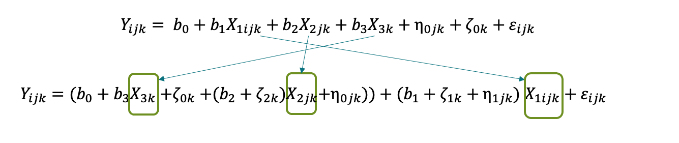
- We might rearrange the ordering of the random effects to better reflect the nesting:
\[
MATHGAIN_{ijk} = b_0 + b_1 SES_{ijk} + b_2 MATHKNOW_{jk} + \zeta_{0k} + \zeta_{1k}SES_{ijk} + \eta_{0jk} + \eta_{1jk}SES_{ijk} + \varepsilon_{ijk}
\]
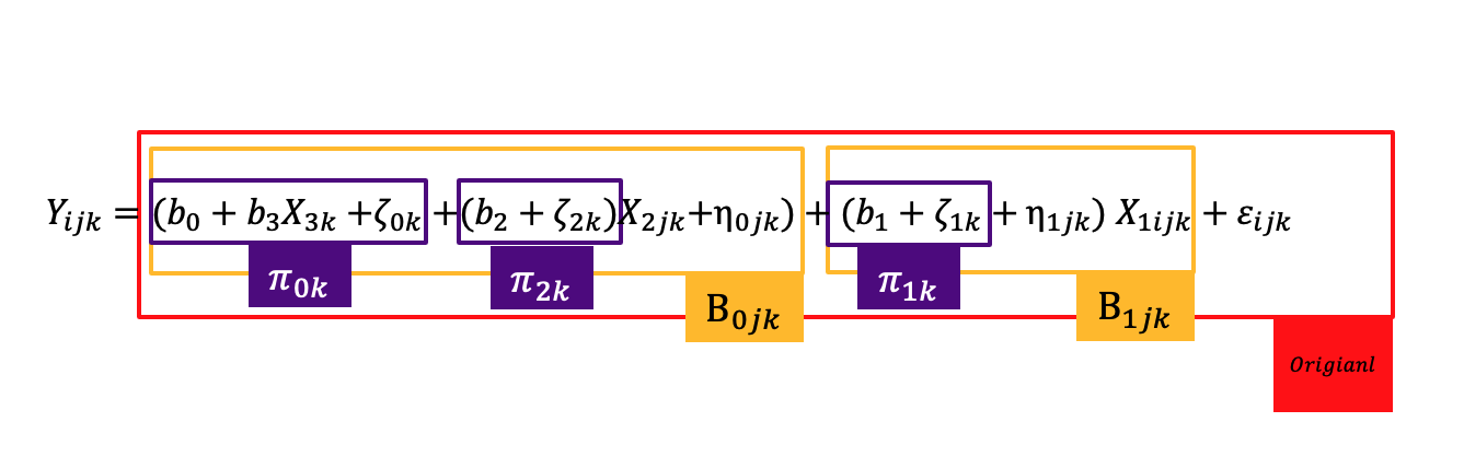
iii.
+ This is the way the model is ‘described’ in most statistical software packages: as a set of ‘regression-like’ fixed effects followed by ‘regression-like’ random effects, in the order of nesting.
+ The challenge with the random effects is that they vary by group, and thus the SYNTAX is a bit different.
+ We can add predictors to the random effects specification as follows: instead of random intercept, +(1|schoolid), a random slope, in SES, would be specified as +(ses||schoolid). In this last bit of notation, the random intercept is included by default, and the effects are assumed uncorrelated (see lmer_useful_guide.pdf in Readings).
+ It is more complicated if different predictor effects vary by different grouping structures. In lmer one can sometimes specify these as crossed effects, but this must be done with care by adjusting identifiers to reflect nesting.
iv. (Simpler) Example I: random return to SES by school, controlling for MATHKNOW as well (and with school and classroom effects), with model:\[ MATHGAIN_{ijk} = b_0 + b_1 SES_{ijk} + b_2 MATHKNOW_{jk} + \eta_{0jk} + \zeta_{0k} + \zeta_{1k} SES_{ijk} + \varepsilon_{ijk} \]
\[ \mbox{ with }\eta_{0jk}\sim N(0,\sigma_{\eta_0}^2),\ \zeta_{0k}\sim N(0,\sigma_{\zeta_0}^2),\ \zeta_{1k}\sim N(0,\sigma_{\zeta_1}^2), \varepsilon_{ijk}\sim N(0,\sigma_\varepsilon ^2),\mbox{ indep.} \]
Code
## Linear mixed model fit by REML. t-tests use Satterthwaite's method ['lmerModLmerTest']
## Formula: mathgain ~ ses + mathknow + (1 | schoolid/classid)
##    Data: dat
##
## REML criterion at convergence: 10684.6
##
## Scaled residuals:
##     Min      1Q  Median      3Q     Max
## -4.3702 -0.6106 -0.0342  0.5357  5.5805
##
## Random effects:
##  Groups           Name        Variance Std.Dev.
##  classid:schoolid (Intercept)  104.64  10.229
##  schoolid         (Intercept)   92.11   9.598
##  Residual                     1018.67  31.917
## Number of obs: 1081, groups:  classid:schoolid, 285; schoolid, 105
##
## Fixed effects:
##              Estimate Std. Error        df t value Pr(>|t|)
## (Intercept)   57.8169     1.5468   91.6576  37.379   <2e-16 ***
## ses            0.8847     1.4602 1039.2449   0.606   0.5447
## mathknow       2.4341     1.3093  211.2083   1.859   0.0644 .
## ---
## Signif. codes:  0 '***' 0.001 '**' 0.01 '*' 0.05 '.' 0.1 ' ' 1
##
## Correlation of Fixed Effects:
##          (Intr) ses
## ses       0.039
## mathknow  0.009 -0.042
Code
## boundary (singular) fit: see help('isSingular')## Linear mixed model fit by REML. t-tests use Satterthwaite's method ['lmerModLmerTest']
## Formula: mathgain ~ ses + mathknow + (0 + ses | schoolid) + (1 | schoolid) +
## (1 | classid)
## Data: dat
##
## REML criterion at convergence: 10684.6
##
## Scaled residuals:
## Min 1Q Median 3Q Max
## -4.3702 -0.6106 -0.0342 0.5356 5.5805
##
## Random effects:
## Groups Name Variance Std.Dev.
## classid (Intercept) 104.64 10.229
## schoolid (Intercept) 92.12 9.598
## schoolid.1 ses 0.00 0.000
## Residual 1018.66 31.917
## Number of obs: 1081, groups: classid, 285; schoolid, 105
##
## Fixed effects:
## Estimate Std. Error df t value Pr(>|t|)
## (Intercept) 57.8169 1.5468 91.6564 37.379 <2e-16 ***
## ses 0.8847 1.4602 1039.2467 0.606 0.5447
## mathknow 2.4341 1.3093 211.2072 1.859 0.0644 .
## ---
## Signif. codes: 0 '***' 0.001 '**' 0.01 '*' 0.05 '.' 0.1 ' ' 1
##
## Correlation of Fixed Effects:
## (Intr) ses
## ses 0.039
## mathknow 0.009 -0.042
## optimizer (nloptwrap) convergence code: 0 (OK)
## boundary (singular) fit: see help('isSingular')- (cont.)
- (cont.)
- The extremely small value for the estimate of \(\sigma_{{\zeta_1}}^2\), in the random-effects portion of the output suggests that we do not have systematic variation in returns to SES at the school level.
- The definitive test is an LRT:
- (cont.)
## Data: dat
## Models:
## fit3: mathgain ~ ses + mathknow + (1 | schoolid/classid)
## fit4: mathgain ~ ses + mathknow + (0 + ses | schoolid) + (1 | schoolid) + (1 | classid)
##      npar   AIC   BIC  logLik deviance Chisq Df Pr(>Chisq)
## fit3    6 10697 10726 -5342.3    10685
## fit4 7 10699 10734 -5342.3 10685 0 1 1- (cont.)
- (cont.)
- We do not identify significant variation in the SES effect over schools (p=1.0)
- It would most likely only be ‘worse’ if we tried to detect variation in SES effects at the classroom level, as these are even smaller units of analysis.
- We do not identify significant variation in the SES effect over schools (p=1.0)
- Example II: Random return to MATHKNOW by school controlling for SES as well (and with school and classroom effects), with model:
- (cont.)
\[
MATHGAIN_{ijk} = b_0 + b_1 SES_{ijk} + b_2 MATHKNOW_{jk} + \eta_{0jk} + \zeta_{0k} + \zeta_{2k} MATHKNOW_{jk} + \varepsilon_{ijk};
\]
\[
\eta_{0jk}\sim N(0,\sigma_{\eta_0}^2),\ \zeta_{0k}\sim N(0,\sigma_{\zeta_0}^2),\ \zeta_{2k} \sim N(0,\sigma_{\zeta_2}^2),\ \varepsilon_{ijk}\sim N(0,\sigma_\varepsilon ^2),\mbox{ indep.}
\]
v.
1. Notice, we use \(\zeta_{2k}\) to refer to the MATHKNOW effect.
## boundary (singular) fit: see help('isSingular')## Linear mixed model fit by REML. t-tests use Satterthwaite's method ['lmerModLmerTest']
## Formula: mathgain ~ ses + mathknow + (0 + mathknow | schoolid) + (1 |
## schoolid) + (1 | classid)
## Data: dat
##
## REML criterion at convergence: 10684.6
##
## Scaled residuals:
## Min 1Q Median 3Q Max
## -4.3702 -0.6106 -0.0342 0.5356 5.5805
##
## Random effects:
## Groups Name Variance Std.Dev.
## classid (Intercept) 104.64 10.229
## schoolid (Intercept) 92.11 9.598
## schoolid.1 mathknow 0.00 0.000
## Residual 1018.67 31.917
## Number of obs: 1081, groups: classid, 285; schoolid, 105
##
## Fixed effects:
## Estimate Std. Error df t value Pr(>|t|)
## (Intercept) 57.8169 1.5468 91.6577 37.379 <2e-16 ***
## ses 0.8847 1.4602 1039.2447 0.606 0.5447
## mathknow 2.4341 1.3093 211.2083 1.859 0.0644 .
## ---
## Signif. codes: 0 '***' 0.001 '**' 0.01 '*' 0.05 '.' 0.1 ' ' 1
##
## Correlation of Fixed Effects:
## (Intr) ses
## ses 0.039
## mathknow 0.009 -0.042
## optimizer (nloptwrap) convergence code: 0 (OK)
## boundary (singular) fit: see help('isSingular')- (cont.)
- (cont.)
- The extremely small value for the estimate of \(\sigma_{\zeta_2}^2\), noted under
mathknowin the random-effects portion of the output, suggests that we do not have systematic variation in returns to MATHKNOW at the school level. - The definitive test is again an LRT:
- The extremely small value for the estimate of \(\sigma_{\zeta_2}^2\), noted under
- (cont.)
## Data: dat
## Models:
## fit3: mathgain ~ ses + mathknow + (1 | schoolid/classid)
## fit5: mathgain ~ ses + mathknow + (0 + mathknow | schoolid) + (1 | schoolid) + (1 | classid)
##      npar   AIC   BIC  logLik deviance Chisq Df Pr(>Chisq)
## fit3    6 10697 10726 -5342.3    10685
## fit5 7 10699 10734 -5342.3 10685 0 1 1- (cont.)
- Example III: We add MATHKIND as a control in the fixed effects. Then we revisit random returns to SES by school controlling for MATHKIND and MATHKNOW (and with school and classroom effects), with model:
\(MATHGAI{N_{ijk}} = {b_0} + {b_1}SE{S_{ijk}} + {b_2}MATHKNO{W_{jk}} + {b_3}MATHKIN{D_{ijk}} + {\eta_{0jk}} + {\zeta_{0k}} + {\zeta_{1k}}SE{S_{ijk}} + {\varepsilon_{ijk}}\),
with \(\eta_{0jk}\sim N(0,\sigma_{\eta_0}^2)\), \(\zeta_{0k}\sim N(0,\sigma_{\zeta_0}^2)\), \({\zeta_{1k}} \sim N(0,\sigma_{\zeta_1^{}}^2)\), and \({\varepsilon_{ijk}} \sim N(0,\sigma_\varepsilon ^2)\), all independent of one another.
- We return to using \(\zeta_{1k}\) to refer to the SES effect.
- We also refit a random intercept model (in schools and classrooms, for subsequent use in the LRT) so that we have a baseline model with the full set of fixed effects. Then, we add random returns to SES.
- We return to using \(\zeta_{1k}\) to refer to the SES effect.
- Example III: We add MATHKIND as a control in the fixed effects. Then we revisit random returns to SES by school controlling for MATHKIND and MATHKNOW (and with school and classroom effects), with model:
\(MATHGAI{N_{ijk}} = {b_0} + {b_1}SE{S_{ijk}} + {b_2}MATHKNO{W_{jk}} + {b_3}MATHKIN{D_{ijk}} + {\eta_{0jk}} + {\zeta_{0k}} + {\zeta_{1k}}SE{S_{ijk}} + {\varepsilon_{ijk}}\),
with \(\eta_{0jk}\sim N(0,\sigma_{\eta_0}^2)\), \(\zeta_{0k}\sim N(0,\sigma_{\zeta_0}^2)\), \({\zeta_{1k}} \sim N(0,\sigma_{\zeta_1^{}}^2)\), and \({\varepsilon_{ijk}} \sim N(0,\sigma_\varepsilon ^2)\), all independent of one another.
Code
## Linear mixed model fit by REML. t-tests use Satterthwaite's method ['lmerModLmerTest']
## Formula: mathgain ~ mathkind + ses + mathknow + (1 | schoolid) + (1 |      classid)
##    Data: dat
##
## REML criterion at convergence: 10331.8
##
## Scaled residuals:
##     Min      1Q  Median      3Q     Max
## -3.4915 -0.6381 -0.0385  0.5666  4.2969
##
## Random effects:
##  Groups   Name        Variance Std.Dev.
##  classid  (Intercept)  79.35    8.908
##  schoolid (Intercept)  78.41    8.855
##  Residual             723.38   26.896
## Number of obs: 1081, groups:  classid, 285; schoolid, 105
##
## Fixed effects:
##              Estimate Std. Error        df t value Pr(>|t|)
## (Intercept)  274.1598    10.5769 1053.1666  25.921  < 2e-16 ***
## mathkind      -0.4642     0.0225 1061.9380 -20.627  < 2e-16 ***
## ses            6.0825     1.2635 1061.6812   4.814 1.69e-06 ***
## mathknow       2.4741     1.1288  228.7374   2.192   0.0294 *
## ---
## Signif. codes:  0 '***' 0.001 '**' 0.01 '*' 0.05 '.' 0.1 ' ' 1
##
## Correlation of Fixed Effects:
##          (Intr) mthknd ses
## mathkind -0.992
## ses       0.200 -0.197
## mathknow -0.004  0.005 -0.040
Code
## Linear mixed model fit by REML. t-tests use Satterthwaite's method ['lmerModLmerTest']
## Formula: mathgain ~ mathkind + ses + mathknow + (0 + ses | schoolid) +
##     (1 | schoolid) + (1 | classid)
##    Data: dat
##
## REML criterion at convergence: 10331.3
##
## Scaled residuals:
##     Min      1Q  Median      3Q     Max
## -3.4954 -0.6360 -0.0513  0.5716  4.3237
##
## Random effects:
##  Groups     Name        Variance Std.Dev.
##  classid    (Intercept)  79.36    8.909
##  schoolid   (Intercept)  76.43    8.743
##  schoolid.1 ses          14.58    3.819
##  Residual               717.24   26.781
## Number of obs: 1081, groups:  classid, 285; schoolid, 105
##
## Fixed effects:
##               Estimate Std. Error         df t value Pr(>|t|)
## (Intercept)  274.88502   10.56248 1045.60363  26.025  < 2e-16 ***
## mathkind      -0.46583    0.02248 1056.71663 -20.725  < 2e-16 ***
## ses            6.05644    1.34261   67.87374   4.511 2.63e-05 ***
## mathknow       2.47291    1.12890  228.97808   2.191   0.0295 *
## ---
## Signif. codes:  0 '***' 0.001 '**' 0.01 '*' 0.05 '.' 0.1 ' ' 1
##
## Correlation of Fixed Effects:
##          (Intr) mthknd ses
## mathkind -0.992
## ses       0.187 -0.182
## mathknow -0.004 0.005 -0.031- (cont.)
- (cont.)
- The value for the estimate of \(\sigma_{\zeta_1}^2\), noted in the row labeled
sesin the random-effects portion of the output suggests that MAYBE we do have systematic variation in returns to SES at the school level. - The definitive test is again an LRT:
- The value for the estimate of \(\sigma_{\zeta_1}^2\), noted in the row labeled
- (cont.)
## Data: dat
## Models:
## fit6: mathgain ~ mathkind + ses + mathknow + (1 | schoolid) + (1 | classid)
## fit7: mathgain ~ mathkind + ses + mathknow + (0 + ses | schoolid) + (1 | schoolid) + (1 | classid)
##      npar   AIC   BIC  logLik deviance Chisq Df Pr(>Chisq)
## fit6    7 10346 10381 -5165.9    10332
## fit7 8 10347 10387 -5165.6 10331 0.519 1 0.4713- (cont.)
- (cont.)
- This suggests that we still cannot identify significant variation in the return to SES (under this additional set of controls).
- (cont.)
- Correlated level and slope
- Until now, we have assumed that every effect is independent of the other, but this could be greatly oversimplifying the situation.
- E.g., in schools with very large school effects (intercepts), maybe the returns to SES are muted, whereas in schools with very negative school effects (intercepts), the returns to SES are quite substantial.
- We can directly model this correlation by introducing a new ‘variance component’ – the correlation between two effects.
- Begin with our model that includes MATHKIND as a control with outcome MATHGAIN:
\[
MATHGAIN_{ijk} = b_0 + b_1 SES_{ijk} + b_2 MATHKNOW_{jk} + b_3 MATHKIND_{ijk} + \eta_{0jk} + \zeta_{0k} + \zeta_{1k}SES_{ijk} + \varepsilon_{ijk}
\]
\[
\eta_{0jk}\sim N(0,\sigma_{\eta_0}^2),\ \zeta_{0k}\sim N(0,\sigma_{\zeta_0}^2),\ \zeta_{1k}\sim N(0,\sigma_{\zeta_1}^2),\ \varepsilon_{ijk}\sim N(0,\sigma_\varepsilon^2),
\]
BUT NOW \(corr(\zeta_{0k},\zeta_{1k}) = \rho_{\zeta_0\zeta_1}\), which may not be zero, and all other pairs of random terms are independent of one another.
- We can use LRTs to determine whether we need a correlation term, but instead, given that we didn’t even ‘need’ a variable return to SES, we test whether adding a correlation between level and slope for SES (by school) improves the model to the point of significance.
- Correlation is the default in R lmer models, so we simply need to condense the schoolid random effects to
+(ses|schoolid)rather than use the two terms+(1|schoolid)+(0+ses|schoolid)as before.
- Until now, we have assumed that every effect is independent of the other, but this could be greatly oversimplifying the situation.
Code
## Linear mixed model fit by REML. t-tests use Satterthwaite's method ['lmerModLmerTest']
## Formula: mathgain ~ mathkind + ses + mathknow + (ses | schoolid) + (1 |      classid)
##    Data: dat
##
## REML criterion at convergence: 10328.9
##
## Scaled residuals:
##     Min      1Q  Median      3Q     Max
## -3.5522 -0.6333 -0.0470  0.5641  4.3032
##
## Random effects:
##  Groups   Name        Variance Std.Dev. Corr
##  classid  (Intercept)  78.34    8.851
##  schoolid (Intercept)  83.17    9.120
##           ses          14.52    3.810   0.75
##  Residual             716.39   26.766
## Number of obs: 1081, groups:  classid, 285; schoolid, 105
##
## Fixed effects:
##               Estimate Std. Error         df t value Pr(>|t|)
## (Intercept)  275.70469   10.54225 1043.58961  26.152  < 2e-16 ***
## mathkind      -0.46763    0.02244 1054.79633 -20.835  < 2e-16 ***
## ses            5.83347    1.35497   67.95606   4.305 5.49e-05 ***
## mathknow       2.24790    1.12740  231.38060   1.994   0.0473 *
## ---
## Signif. codes:  0 '***' 0.001 '**' 0.01 '*' 0.05 '.' 0.1 ' ' 1
##
## Correlation of Fixed Effects:
##          (Intr) mthknd ses
## mathkind -0.991
## ses       0.197 -0.171
## mathknow -0.008  0.011 -0.023
Code
## Data: dat
## Models:
## fit6: mathgain ~ mathkind + ses + mathknow + (1 | schoolid) + (1 | classid)
## fit8: mathgain ~ mathkind + ses + mathknow + (ses | schoolid) + (1 | classid)
##      npar   AIC   BIC  logLik deviance Chisq Df Pr(>Chisq)
## fit6    7 10346 10381 -5165.9    10332
## fit8 9 10347 10392 -5164.5 10329 2.845 2 0.2411- (cont.)
- The value for the estimate of \(\sigma_{\zeta_1}^2\), noted in the line with
sesis about the same in this model. - The estimate of \(corr({\zeta_{0k}},{\zeta_{1k}}) = {\rho_{{\zeta_0}{\zeta_1}}}\), 0.75, is to the right of the estimates for the intercept and slope random effects.
- Confidence intervals can be generated with a separate command (
confintinlme4package; yields them in terms of s.d. units – commented out), but CIs for variance terms are so controversial as to never be reported by some researchers. - CIs are useful for correlations because they may be positive or negative. However, for this model, we commented out the calls and suppressed the output due to speed and readability considerations. If you run it, those listed as .sig03 and .sig04 are associated with the
sesterm, and suggest no information about it (-1 or +1 correlations are problematic - a red flag). The warnings that would fill a page suggest this is a poorly specified model.
- Confidence intervals can be generated with a separate command (
- The LRT, still ‘rejects’ the need for the 2 new parameters in this model, compared to a simpler, level-effects (intercepts) only version.
- CONCLUSION: we tried pretty hard to identify varying returns to a predictor, but could not do so. We may be more successful with other data and models.
- The value for the estimate of \(\sigma_{\zeta_1}^2\), noted in the line with
3.2 Sampling variance & Wald tests; random slopes (redux)
- There is an important distinction between sampling variation of parameter estimates and variation between groups (random effects). We build intuition for this through the derivation of a Wald test.
- Say we have two nested models, M1 with fixed effect parameters \(({b_0},{b_1},{b_2})\) and M2 with fixed effect parameters \(({b_0},{b_1},{b_2},{b_3},{b_4},{b_5})\), and we wish to determine whether the new parameters \(({b_3},{b_4},{b_5})\) are significant as a block.
- NOTE: we can this with a LRT. But we learn something important by examining an alternative approach.
- A test of \(H_0: {b_3} = {b_4} = {b_5} = 0\) is more complicated than a z-test, which is one-dimensional. The following generalization of a z-test to more than one parameter is called a Wald test.
- We now describe a concrete example in which we are faced with this inferential problem: Using the classroom data and MATHGAIN outcome, we fit a model with random classroom and school effects, along with two subject-level (SES and MINORITY) and three classroom-level (MATHKNOW, MATHPREP and YEARSTEA) predictors. The goal is to evaluate whether the classroom-level predictors are significant, as a block. Here is the R code for the full model:
- Say we have two nested models, M1 with fixed effect parameters \(({b_0},{b_1},{b_2})\) and M2 with fixed effect parameters \(({b_0},{b_1},{b_2},{b_3},{b_4},{b_5})\), and we wish to determine whether the new parameters \(({b_3},{b_4},{b_5})\) are significant as a block.
Code
## Linear mixed model fit by REML. t-tests use Satterthwaite's method ['lmerModLmerTest']
## Formula: mathgain ~ ses + minority + mathknow + mathprep + yearstea +
##     (1 | schoolid) + (1 | classid)
##    Data: dat
##
## REML criterion at convergence: 10676.7
##
## Scaled residuals:
##     Min      1Q  Median      3Q     Max
## -4.3728 -0.6085 -0.0331  0.5384  5.5357
##
## Random effects:
##  Groups   Name        Variance Std.Dev.
##  classid  (Intercept)  104.48  10.221
##  schoolid (Intercept)   86.04   9.276
##  Residual             1020.54  31.946
## Number of obs: 1081, groups:  classid, 285; schoolid, 105
##
## Fixed effects:
##              Estimate Std. Error        df t value Pr(>|t|)
## (Intercept)   50.3603     4.3606  266.7169  11.549   <2e-16 ***
## ses            1.0518     1.4911 1062.9521   0.705   0.4807
## minority       0.8093     2.7827  486.3360   0.291   0.7713
## mathknow       2.4438     1.3183  208.5402   1.854   0.0652 .
## mathprep       2.3771     1.3207  181.0698   1.800   0.0735 .
## yearstea       0.0595     0.1348  203.2240   0.441   0.6595
## ---
## Signif. codes:  0 '***' 0.001 '**' 0.01 '*' 0.05 '.' 0.1 ' ' 1
##
## Correlation of Fixed Effects:
##          (Intr) ses    minrty mthknw mthprp
## ses      -0.104
## minority -0.464  0.198
## mathknow -0.071 -0.012  0.151
## mathprep -0.726  0.055  0.009  0.003
## yearstea -0.268 -0.034 0.041 0.012 -0.167- (cont.)
- We begin by REVIEWING the evaluation of whether one of the predictors is significant. How is this done?
- When we fit a model, we get a set of parameter estimates and standard errors for each.
- Standard error is an estimate of the variability of the parameter estimate. If we were to gather similar data from this population, we would expect the fixed effect parameter estimates to vary from sample to sample.
- Here is some R code that simulates 100 simple linear regressions in which the beta is known to be 1, but varies in any particular sample (we generate samples from a known population mechanism):
- Standard error is an estimate of the variability of the parameter estimate. If we were to gather similar data from this population, we would expect the fixed effect parameter estimates to vary from sample to sample.
Code
- (cont.)
- (cont.)
- We reproduce the (edited) results from fitting the first two regressions here:
- (cont.)
##
## Call:
## lm(formula = y[[1]] ~ x[[1]])
##
## Residuals:
##     Min      1Q  Median      3Q     Max
## -1.8768 -0.6138 -0.1395  0.5394  2.3462
##
## Coefficients:
##             Estimate Std. Error t value Pr(>|t|)
## (Intercept) -0.03769    0.09699  -0.389    0.698
## x[[1]]       0.99894    0.10773   9.273 4.58e-15 ***
## ---
## Signif. codes:  0 '***' 0.001 '**' 0.01 '*' 0.05 '.' 0.1 ' ' 1
##
## Residual standard error: 0.9628 on 98 degrees of freedom
## Multiple R-squared:  0.4674, Adjusted R-squared:  0.4619
## F-statistic: 85.99 on 1 and 98 DF, p-value: 4.583e-15##
## Call:
## lm(formula = y[[2]] ~ x[[2]])
##
## Residuals:
## Min 1Q Median 3Q Max
## -2.74179 -0.56139 -0.01749 0.67973 1.84843
##
## Coefficients:
## Estimate Std. Error t value Pr(>|t|)
## (Intercept) 0.04845 0.09910 0.489 0.626
## x[[2]] 1.10622 0.09626 11.492 <2e-16 ***
## ---
## Signif. codes: 0 '***' 0.001 '**' 0.01 '*' 0.05 '.' 0.1 ' ' 1
##
## Residual standard error: 0.9906 on 98 degrees of freedom
## Multiple R-squared: 0.574, Adjusted R-squared: 0.5697
## F-statistic: 132.1 on 1 and 98 DF, p-value: < 2.2e-16- (cont.)
- (cont.)
- The estimate of beta associated with X is 0.999 and its standard error is estimated to be 0.108. We wrote our simulation so that (population) beta is 1; it was estimated to be nearly the same in this sample.
- The results of the second run from simulated data are similar, but not identical. Note how the estimate of beta for the X is now 1.106, and the std. err. is estimated to be 0.096. The values change from sample to sample.
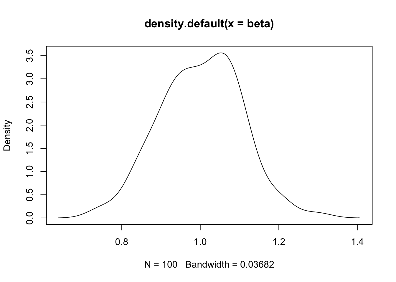
- We repeated this exercise 100 times, and can evaluate the std. dev. of the 100 betas for X estimated from the samples. The observed std. dev. of those 100 betas is an estimate of the std. err.5. We get the value 0.103 in our simulations. Theory would give the value 0.10, based on our DGP and sample size.
- We have an estimate of the std. err. of the estimate of the beta for X, based on our simulations, but this is slightly different from the s.e. that is derived from the ‘output’ in our first two simulations (we have to rely on theory to know the distribution in a real problem with one sample). Thus, std. err. computations in standard regression are based on MLE (asymptotic) theory.6 We have been exploring the same concept empirically via simulations.
- Here is the density plot depicting the sampling distribution of the beta for X, based on the simulation:
- (cont.)
- We now revisit our example, with the simple goal of first evaluating the significance of MATHPREP, and then the significance of a block of classroom-level predictors (recall the results):
## Linear mixed model fit by REML. t-tests use Satterthwaite's method ['lmerModLmerTest']
## Formula: mathgain ~ ses + minority + mathknow + mathprep + yearstea +
##     (1 | schoolid) + (1 | classid)
##    Data: dat
##
## REML criterion at convergence: 10676.7
##
## Scaled residuals:
##     Min      1Q  Median      3Q     Max
## -4.3728 -0.6085 -0.0331  0.5384  5.5357
##
## Random effects:
##  Groups   Name        Variance Std.Dev.
##  classid  (Intercept)  104.48  10.221
##  schoolid (Intercept)   86.04   9.276
##  Residual             1020.54  31.946
## Number of obs: 1081, groups:  classid, 285; schoolid, 105
##
## Fixed effects:
##              Estimate Std. Error        df t value Pr(>|t|)
## (Intercept)   50.3603     4.3606  266.7169  11.549   <2e-16 ***
## ses            1.0518     1.4911 1062.9521   0.705   0.4807
## minority       0.8093     2.7827  486.3360   0.291   0.7713
## mathknow       2.4438     1.3183  208.5402   1.854   0.0652 .
## mathprep       2.3771     1.3207  181.0698   1.800   0.0735 .
## yearstea       0.0595     0.1348  203.2240   0.441   0.6595
## ---
## Signif. codes:  0 '***' 0.001 '**' 0.01 '*' 0.05 '.' 0.1 ' ' 1
##
## Correlation of Fixed Effects:
##          (Intr) ses    minrty mthknw mthprp
## ses      -0.104
## minority -0.464  0.198
## mathknow -0.071 -0.012  0.151
## mathprep -0.726  0.055  0.009  0.003
## yearstea -0.268 -0.034 0.041 0.012 -0.167- (cont.)
- The std. err. for MATHPREP is 1.321. Given a parameter estimate \(\hat{b}_4\) of 2.377, the t-test has value 1.8 and corresponding (two-sided) p-value 0.074. The key question is where did we get the s.e. and p-value?
- The null is \(H_0: b_4=0\) (MATHPREP is the \(4^{th}\) predictor in our list), and the test statistic based on this is \(z = \frac{\hat b_4 - 0}{\mbox{s.e.}(\hat b_4)}\) (this can be thought of as ‘standardizing’ the estimate). Reminder: we put ‘hats’ on the parameters because they are estimated from the data under the model.
- Now the value for t=1.8 (the test statistic) comes directly from the formula: (2.38-0)/1.32.
- Our theory for MLEs tells us that under \(H_0\), \(t \sim N(0,1)\) (t is distributed approximately as a standard normal, at least in large samples (this is what is meant by asymptotically).
- Then \(\Pr (\left| z \right| > 1.80) = 0.07\).
- REMINDER: Our regression parameter 2.38 is the population-level effect of MATHPREP on any individual, no matter what classroom or school (these other effects have been ‘netted out’).
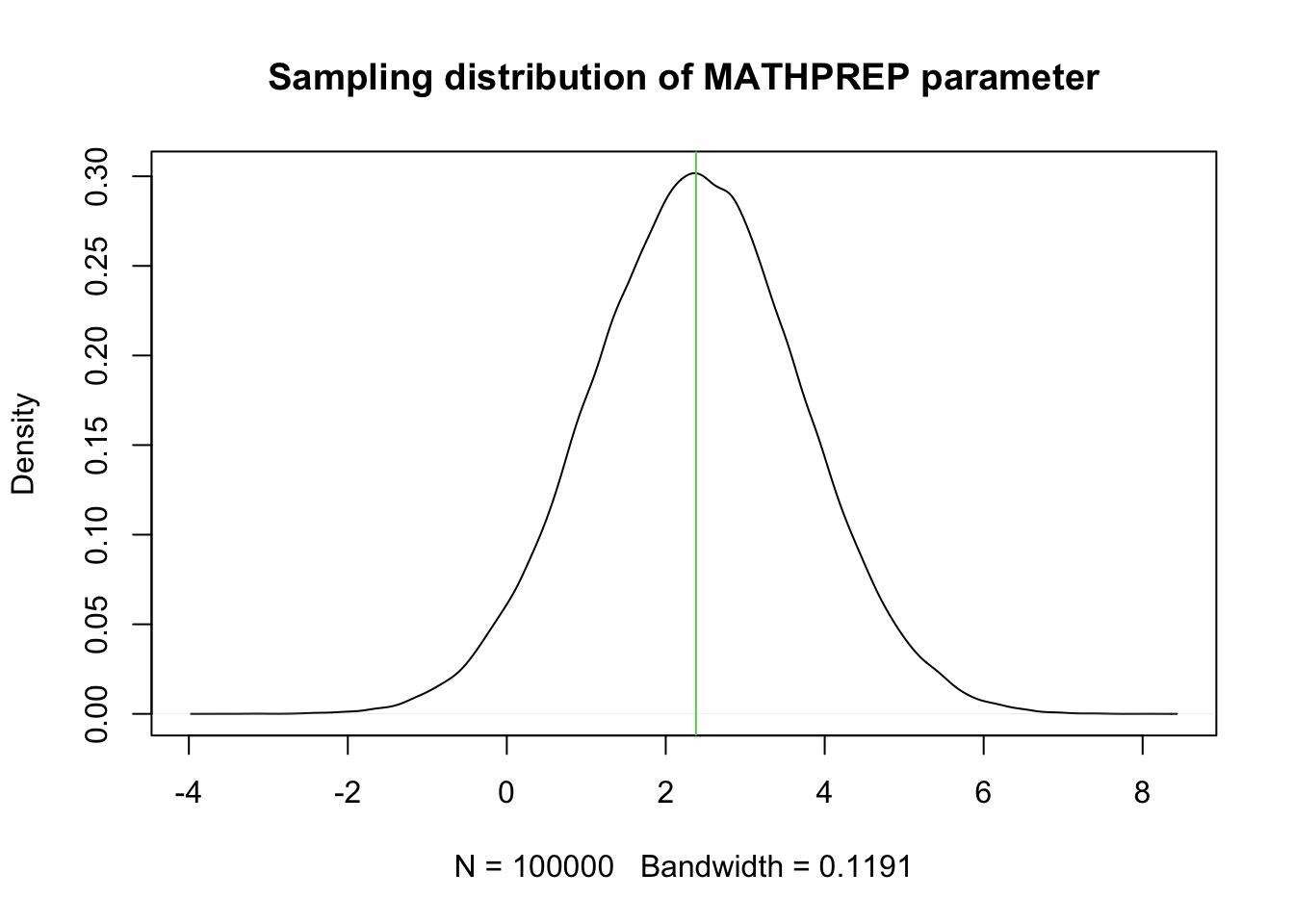
1. The std. err. of a regression parameter (1.32 in this case) describes the uncertainty in that estimate.7 2. Variation in this parameter occurs through sampling variability: in different samples, we might estimate a different ‘effect’ for MATHPREP. Here is the idealized distribution of parameter estimates we would expect for MATHPREP in data from the same population (this is simply a normal distribution centered at the estimated value, with std. dev. equal to the estimated std. err.):- This is the theoretical distribution of the single fixed effect parameter estimate (normal, mean 2.38, std.dev. 1.32 –why do I write std.dev., not std.err.?).
- This type of variation is distinctly different from that reflected in variance components: the variance of the random effect. The latter describes variation from group to group in a latent variable. We need to be clear on this distinction.
- This is the theoretical distribution of the single fixed effect parameter estimate (normal, mean 2.38, std.dev. 1.32 –why do I write std.dev., not std.err.?).
- The std. err. for MATHPREP is 1.321. Given a parameter estimate \(\hat{b}_4\) of 2.377, the t-test has value 1.8 and corresponding (two-sided) p-value 0.074. The key question is where did we get the s.e. and p-value?
Code
- How can we possibly evaluate the null \(H_0: {b_3} = {b_4} = {b_5} = 0\) (other than using an LRT)?
i. The approach that we use in fitting MLMs, maximum likelihood estimation, provides us with theory-based estimates of the std. err. of each parameter estimate, but it tells us something more as well.
ii. If we look at two parameter estimates simultaneously, we begin to see that there is more information about the uncertainty. Start with \(\hat b_3\) and \(\hat b_4\). Under theory for MLEs, we have expressions for: \(\mbox{s.e.}(\hat b_3)\), \(\mbox{s.e.}(\hat b_4)\) and \(corr({\hat b_3},{\hat b_4})\). We will use the correlation in the assessment of a multivariate null hypothesis.
iii. We have a way to express all of these relationships in a covariance matrix, which is a fancy form of a correlation table (scaled by variances). In our example, with three parameters, theory tells us that \(({\hat b_3},{\hat b_4},{\hat b_5})' \sim N(({b_3},{b_4},{b_5})',\Sigma )\), with \[\Sigma = \left( {\begin{array}{*{20}{c}} {\sigma_3^2}&{{\sigma_3}{\sigma_4}{\rho_{34}}}&{{\sigma_3}{\sigma_5}{\rho_{35}}}\\ {{\sigma_3}{\sigma_4}{\rho_{34}}}&{\sigma_4^2}&{{\sigma_4}{\sigma_5}{\rho_{45}}}\\ {{\sigma_3}{\sigma_5}{\rho_{35}}}&{{\sigma_4}{\sigma_5}{\rho_{45}}}&{\sigma_5^2} \end{array}} \right)\] where we use the ‘hat’ symbol for the estimates. Without a ‘hat’, the parameters are taken to be the ‘true’ values.
iv. Under \(H_0: {b_3} = {b_4} = {b_5} = 0\), \(({b_3},{b_4},{b_5}){\Sigma ^{ - 1}}({b_3},{b_4},{b_5})' \sim \chi_3^2\). The expression is just a (complicated) weighted average of all of the terms in \({\Sigma ^{ - 1}}\).- \({\Sigma ^{ - 1}}\) is \(\Sigma\)’s matrix inverse. It’s the reciprocal if the matrix has one element.8
- Believe it or not, when we are testing a single parameter, we are using this formula, only we don’t “square” the left hand side (chi-sq is a squared standard normal).
- To construct this test manually is a bit of work, but we do it below. R libraries tend to rely on LRTs and this requires that the models to be rerun using ML not REML (if we use the anova command). To get around this, we have to rely on some functions in other libraries (similar to using the
ranovafunction from lmerTest for tests of random effects). The library with a generic Wald test built in is known ascarand the functionlinearHypothesis.- Fortunately, an estimate of \(\Sigma\) is readily available as part of the estimation procedure in most packages.
Code
## 6 x 6 Matrix of class "dpoMatrix"
##             (Intercept)          ses    minority    mathknow    mathprep     yearstea
## (Intercept)  19.0145718 -0.676083405 -5.62962890 -0.40577135 -4.18167950 -0.157597693
## ses          -0.6760834  2.223340244  0.82089335 -0.02334611  0.10737993 -0.006776006
## minority     -5.6296289  0.820893348  7.74319774  0.55570751  0.03190917  0.015475193
## mathknow     -0.4057713 -0.023346107  0.55570751  1.73782290  0.00529564  0.002097740
## mathprep     -4.1816795  0.107379927  0.03190917  0.00529564  1.74428428 -0.029686428
## yearstea -0.1575977 -0.006776006 0.01547519 0.00209774 -0.02968643 0.018178880- (cont.)
- Estimates of the squared std. err. of each parameter estimate are given by the diagonal terms. E.g., 1.7443 is the squared version of the s.e. for MATHPREP.9
- We now separate out the variances and covariances associated with the three classroom-level effects only, and then manually compute the Wald statistic described above, followed by an easier way.
## 3 x 3 Matrix of class "dsyMatrix"
##            mathknow    mathprep    yearstea
## mathknow 1.73782290  0.00529564  0.00209774
## mathprep 0.00529564  1.74428428 -0.02968643
## yearstea 0.00209774 -0.02968643 0.01817888##
## This is the inverse:## 3 x 3 Matrix of class "dsyMatrix"
## mathknow mathprep yearstea
## mathknow 0.575527652 -0.002959856 -0.07124614
## mathprep -0.002959856 0.589705377 0.96334071
## yearstea -0.071246137 0.963340711 56.59026216## 1 x 1 Matrix of class "dgeMatrix"
## [,1]
## [1,] 7.187268##
## Easier Wald test:## Linear hypothesis test
##
## Hypothesis:
## mathknow = 0
## mathprep = 0
## yearstea = 0
##
## Model 1: restricted model
## Model 2: mathgain ~ ses + minority + mathknow + mathprep + yearstea +
## (1 | schoolid) + (1 | classid)
##
## Df Chisq Pr(>Chisq)
## 1
## 2 3 7.1873 0.06616 .
## ---
## Signif. codes: 0 '***' 0.001 '**' 0.01 '*' 0.05 '.' 0.1 ' ' 1- (cont.)
- To be clear, the matrix \[ \hat \Sigma = \left( {\begin{array}{*{20}{c}} {1.738}&{.005}&{.002}\\ {.005}&{1.744}&{ - .030}\\ {.002}&{ - .030}&{.018} \end{array}} \right) \]
(we put a hat on because it is estimated from the data) reflects our simultaneous uncertainty about three parameters, \((\hat b_3,\hat b_4,\hat b_5)'\).
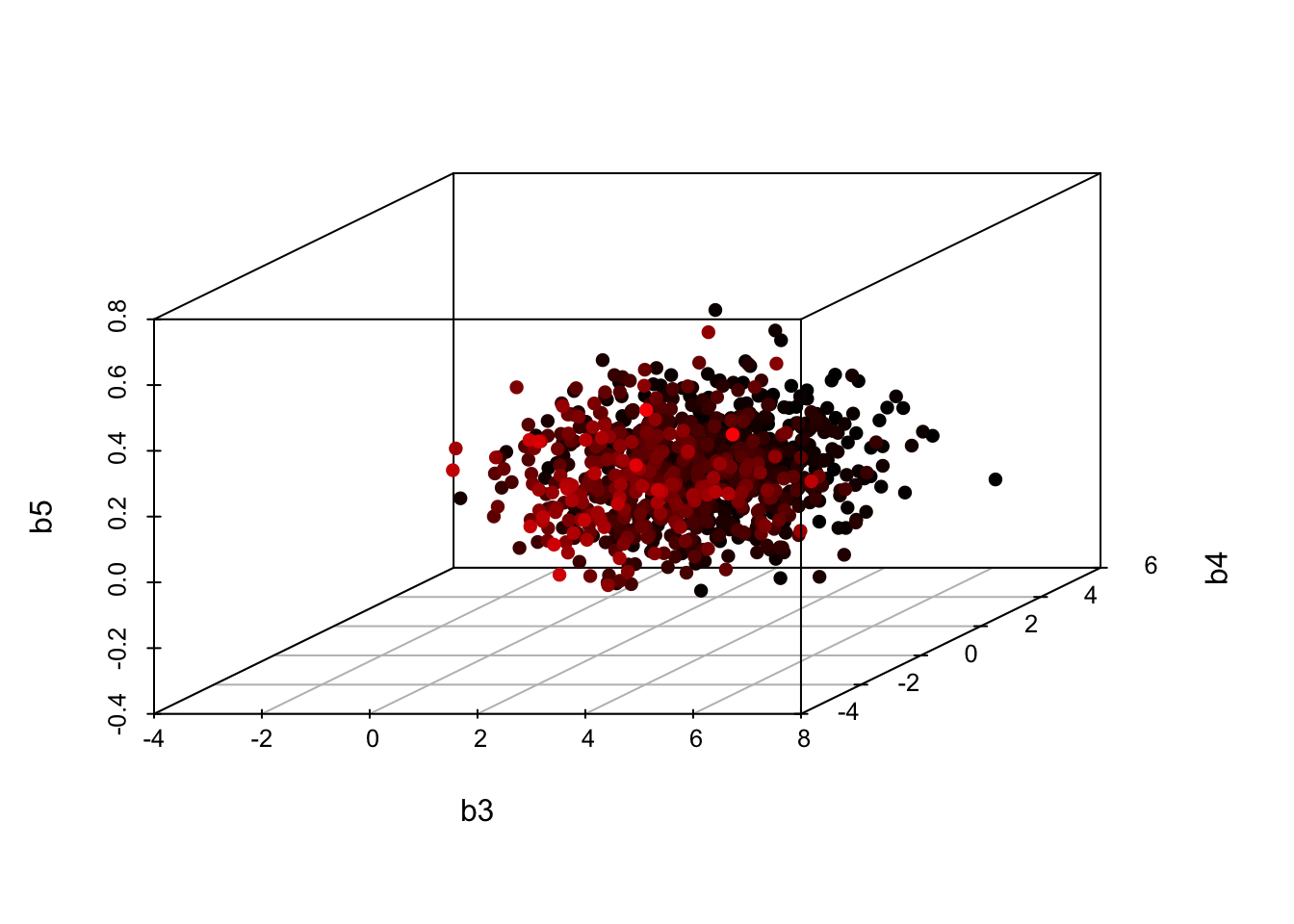
1. Their distribution (in repeated samples from data from this population) is multivariate normal, centered at the estimates, \(({\hat b_3},{\hat b_4},{\hat b_5})'\). Below is a simulation of the estimates you can expect from similar samples:
Code
- (cont.)
(cont.) 2. Most estimates are expected to lie near the center, which is the MLE. To the extent that some estimates deviate from that center, they move together, as a group of three, in a manner governed by this multivariate normal distribution. e. Uncertainty in \(b_4\) (the MATHPREP coefficient) is very different from the variance in a random slope term centered on \(b_4\).
Uncertainty in \(b_4\) comes from sampling variation, not differences between groups. For any given dataset, we have one estimate of \(b_4\) and we expect that it will vary from sample to sample.
- A large std. err. around a regression parameter may lead to us declaring it non-significant, which is another way of saying that it was likely a ‘fluke’ – signs may shift, etc., so we had better not ‘believe’ it too much.
A random slope associated with MATHPREP varies from group to group; this is different from sampling variation. Let’s look a little more closely at a model with variation across groups in slope terms: \[ MATHGAIN_{ijk} = b_0 + b_1 SES_{ijk} + b_2 MINORITY_{ijk} + b_3 MATHKNOW_{jk} + b_4 MATHPREP_{jk} \] \[ +{b_5}YEARSTEA_{jk} + \eta_{0jk} + \zeta_{0k} + \zeta_{4k} MATHPREP_{jk} +\varepsilon_{ijk} \] \[ \eta_{0jk}\sim N(0,\sigma_{\eta_0}^2),\ \zeta_{0k}\sim N(0,\sigma_{\zeta_0}^2),\ \zeta_{4k}\sim N(0,\sigma_{\zeta_4}^2),\ \varepsilon_{ijk}\sim N(0,\sigma_\varepsilon^2) \mbox{ indep.} \]
The variance component \(\sigma_{\zeta_4}^2\)is not a (squared) std. error. It is part of a multi-level model, specifying how much between school-variation can be attributed to different returns to MATHPREP.
- For school k, we predict that the return to MATHPREP is \({\hat b_4} + {\zeta_{4k}}\), not simply \(\hat b_4\), and this sum varies from school to school.
- When \(\hat \sigma_{{\zeta_4}}^2\) is large, \(\zeta_{4k}\) will take on a large range of values.
- Say \(\hat \sigma_{{\zeta_4}}^2=4\). Then ignoring sampling variation, and looking at between-school variation, \({\hat b_4} + {\zeta_{4k}} \sim N({\hat b_4},{2^2})\), so we would expect 68% of the effect of MATHPREP (its combined fixed+random coefficient) to lie within one s.d. of the mean, or between \({\hat b_4} - 2\) and \({\hat b_4} + 2\).
- These are different returns to MATHPREP in different schools, just like we have different mean levels (intercept differences) for different schools.
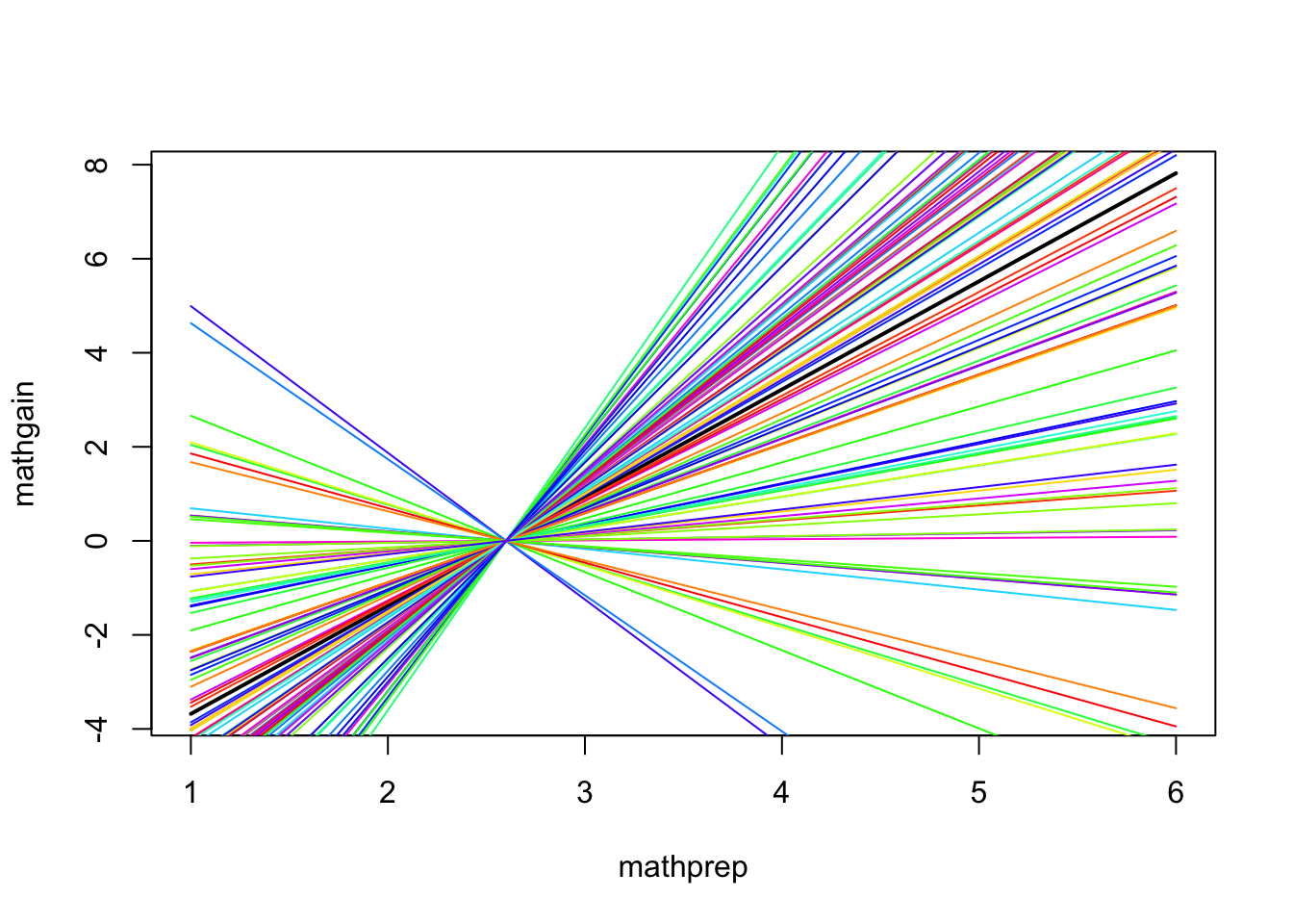
- \(\hat b_4\) is about 2.3. If \(\hat \sigma_{{\zeta_4}}^2=4\), then we would expect the relationship between MATHGAIN and MATHPREP to vary, by school, in a manner depicted by this graphic:
Code
- (cont.)
- (cont.)
- All of the colors represent different schools, so these are varying returns to MATHPREP (we centered things so that all lines pass though the point (\(\overline{MATHPREP}\),0).
- This example was exaggerated slightly (and idealized) to make a point about the impact of \(\hat \sigma_{{\zeta_4}}^2\). The actual model fit shows a slightly smaller random return to MATHPREP:
- (cont.)
Code
## Data: dat
## Models:
## fit1: mathgain ~ ses + minority + mathknow + mathprep + yearstea + (1 | schoolid) + (1 | classid)
## fit2: mathgain ~ ses + minority + mathknow + mathprep + yearstea + (0 + mathprep | schoolid) + (1 | schoolid) + (1 | classid)
## npar AIC BIC logLik deviance Chisq Df Pr(>Chisq)
## fit1 9 10695 10740 -5338.4 10677
## fit2 10 10696 10746 -5338.2 10676 0.2454 1 0.6203- (cont.)
- (cont.)
- But the LRT suggests that this is not significant; that’s why we’re saying it was ‘idealized’ (useful for expository purposes only).
- (cont.)
3.3 Appendix
[Additional support material on chapter 3 concepts]
Images from the Jamboard slides “Jamboard: MLM Module 3”
Slides are directly sourced from the slides “W3_slides”
Need of randome slope
Tracing errors
Level notation
3.4 Coding
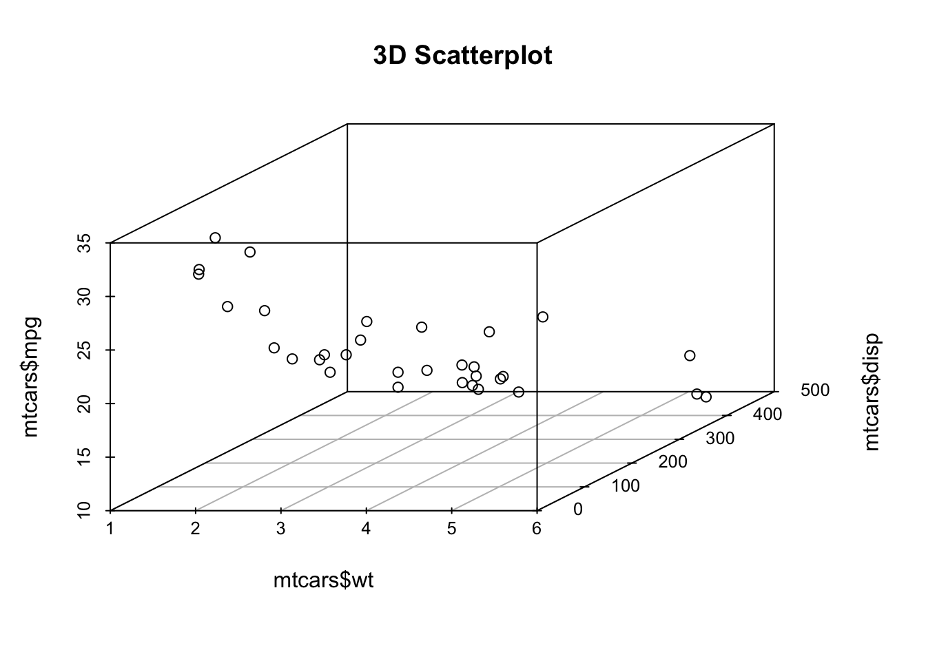
lmer()advancedlinearHypothesis()rmvnorm()scatterplot3d()
lmer()advanced (??)Base model \(MATHGAIN_{ijk} = b_0 + b_1SES_{ijk} + b_2MATHKNOW_{jk} + \eta_{jk} + \zeta_{k} + \epsilon_{ijk}\)
- nested form lmer(mathgain ~ ses + mathknow + (1|schoolid/classid), data=classroom)
- last term uniquely identifies the classroom effect lmer(mathgain ~ ses + mathknow + (1|schoolid) + (1|schoolid:classid), data=classroom)
- write the error terms separately (could be ambiguous) lmer(mathgain ~ ses + mathknow + (1|schoolid) + (1|classid), data=classroom)
linearHypothesis()is a function for testing a linear hypothesis fromcarlibrary; It uses Wald chi-square tests for the fixed effects in mixed-effects models. It has arguments as follows:model: fitted model object
hypothesis.matrix: matrix giving linear combination of coefficients
rhs: right-hand-side vector for hypothesis
Code
## Linear hypothesis test
##
## Hypothesis:
## mathknow = 0
## mathprep = 0
## yearstea = 0
##
## Model 1: restricted model
## Model 2: mathgain ~ ses + minority + mathknow + mathprep + yearstea +
##     (1 | schoolid) + (1 | classid)
##
##   Df  Chisq Pr(>Chisq)
## 1
## 2  3 7.1873    0.06616 .
## ---
## Signif. codes: 0 '***' 0.001 '**' 0.01 '*' 0.05 '.' 0.1 ' ' 1rmvnorm()is a function to create a data with multivariate normal distribution given a mean vector frommvtnormlibrary. It has arguments as follows:n: number of observation to generate
mean: mean vector
sigma: positive covariance matrix
Code
##      mathknow    mathprep    yearstea
## [1,] 1.430021  4.41927057 -0.07967174
## [2,] 3.876337  2.27303000 -0.12550486
## [3,] 2.678260 -0.09822279  0.23257796
## [4,] 3.007793  0.43737464  0.09507983
## [5,] 2.232096  0.69185882 -0.04831520
## [6,] 3.111969 1.93463563 0.05954906scatterplot3d()is a function to plot a 3-dimensional scatterplot with 3 variables fromscatterplot3dlibrary. Additionally,rgllibrary can be helpful in visualizing 3-dimensional scatterplot interactively. t has arguments as follows:x: the coordinates of points in x-axis
y: the coordinates of points in y-axis
z: the coordinates of points in z-axis
col: colors of points
main: a title for the plot
Code
3.5 Quiz
3.5.1 Self-Assessment
Use “Quiz-W3: Exercise” to submit your answers.
- Given this multi-level equation:
\[ MATHGAIN_{ijk} = \beta_{0jk}SES_{ijk} + b_2MATHKNOW_{jk} + \epsilon_{ijk} \] Write down all necessary equations for \(\beta_{0jk}, \beta_{1jk}\) so that we have as follows:
1-A: Random intercepts at the school and classroom level
1-B: Random slopes in \(SES\) at the classroom level
1-C: What parameter represents the fixed effect (or average across the population) for \(SES\)? For \(MATHKNOW\)?
1-D: What would happen if \(\beta_{ijk}\) were replaced by \(\beta_{1k}\) in the level 1 equation?
1-E: The equation in iv. has four random terms. Name these terms with its function (random intercepts, slopes or neither?)
1-F: What is the level at which each effect varies?
1-G: Write the equation in iv. using three level notation (there are strict rules for each level). Be sure to include model assumptions as well.
3.5.2 Lab Quiz
- Review the material in the Rshiny app “Week3: Handout3 Activity” and then answer these questions on the google form “Quiz-W3: Exercise”
3.5.3 Homework
- Homework is presented as the last section of the Rshiny app “Week3: Handout3 Activity”.
- Follow instructions there (fill out this form “Quiz-W3: Exercise” ) and hand in your code on Brightspace
We are of course assuming that treatment did not change the sex ratios.↩︎
At a minimum, we have to assume that litter size is not affected by treatment.↩︎
Independence between slope and intercept within classroom is a strong assumption that can be changed to allow correlation.↩︎
The standard error is the standard deviation of the sampling distribution of a statistic (such as a mean or regression coefficient)↩︎
For those familiar with matrix notation, in linear regression, if \(Y = X\beta + \varepsilon ;\;\varepsilon \sim N(0,\sigma_\varepsilon ^2)\), then \(\Sigma = {(X'X)^{ - 1}}\sigma_\varepsilon ^2\), and recall that the columns of X are known – they are a column of ones for the constant followed by a separate column for each of the predictors.↩︎
The covariances are in the off-diagonal terms and represent dependency between parameter estimates (from sample to sample).↩︎