Chapter 5 : Level Notation, Psuedo-R^2, Nested Longitudinal Data
5.1 Level Notation and targeting variation – one example
- Example of “Bryk/Raudenbush Level Notation” using Rat pup data
- Data description: 30 female rats were randomly assigned to receive one of three doses (none control, low and high) of an experimental compound expected to change birthweight. Several things happened during the study:
- Three of the rats given high doses died
- The number of pups per litter varied from 2 to 18
- …the data are thus unbalanced in two ways
- Predictors / identifiers:
- Pup-based (level 1):
- Weight (birth weight – the outcome)
- Sex (male, female)
- Litter-based (level 2 – these differ at the group level):
- Treatment (control, high, low, in that order)
- Litsize: litter size
- Litter: litter ID
- Pup-based (level 1):
- First fit an unconditional means model M0; here it is, in level notation, for pup \(i\) in litter \(j\):
- Data description: 30 female rats were randomly assigned to receive one of three doses (none control, low and high) of an experimental compound expected to change birthweight. Several things happened during the study:
\[\begin{align*} & \mbox{Level 1: } WEIGHT_{ij} = \beta_{0j} + \varepsilon_{ij} \\ & \mbox{Level 2: } \beta_{0j} = b_{00} + \zeta_{0j} \\ & \zeta_{0j}\sim N(0,\sigma_{\zeta_0}^2),\ \varepsilon_{ij}\sim N(0,\sigma_\varepsilon^2), \mbox{ indep.} \end{align*}\] c. (cont.) i. NOTE: the extra zeros are part of the notation. The 1st subscript links all others to that equation on levels 2 and above.
## Loading required package: lmeTest## Warning in library(package, lib.loc = lib.loc, character.only = TRUE, logical.return = TRUE, :
## there is no package called 'lmeTest'Code
## Linear mixed model fit by REML. t-tests use Satterthwaite's method ['lmerModLmerTest']
## Formula: weight ~ 1 + (1 | litter)
##    Data: ratdat
##
## REML criterion at convergence: 468.7
##
## Scaled residuals:
##     Min      1Q  Median      3Q     Max
## -7.2978 -0.4358 -0.0119  0.4837  3.1972
##
## Random effects:
##  Groups   Name        Variance Std.Dev.
##  litter   (Intercept) 0.3004   0.5481
##  Residual             0.1963   0.4431
## Number of obs: 322, groups:  litter, 27
##
## Fixed effects:
##             Estimate Std. Error      df t value Pr(>|t|)
## (Intercept)   6.1953     0.1091 24.1543   56.79   <2e-16 ***
## ---
## Signif. codes: 0 '***' 0.001 '**' 0.01 '*' 0.05 '.' 0.1 ' ' 1- (cont.)
d. The variance components are: \(\sigma_{{\zeta _0}}^2 = 0.30\); \(\sigma _\varepsilon ^2 = 0.20\). There is more between-litter variation than within.
- There were two treatment levels associated with the dosage, and it is clearly of interest to see whether they had an effect. This will be our model M1. These are entered in level 2, since treatment was assigned at the litter-level:
\[\begin{align*} & \mbox{Level 1: } WEIGHT_{ij} = \beta_{0j} + \varepsilon_{ij} \\ & \mbox{Level 2: } \beta_{0j} = b_{00} + b_{01}TREAT2_j + b_{02}TREAT3_j + \zeta_{0j} \\ & \zeta_{0j}\sim N(0,\sigma_{\zeta_0}^2),\ \varepsilon_{ij}\sim N(0,\sigma_\varepsilon^2), \mbox{ indep.} \end{align*}\]
- (cont.)
- TREATn is an indicator for treatment code 2 (high) or 3 (low).
- Note: the reference is the control group, but treatment codes are based on the alphabetical ordering of ‘High’ and ‘Low’.
- TREATn is an indicator for treatment code 2 (high) or 3 (low).
## Linear mixed model fit by REML. t-tests use Satterthwaite's method ['lmerModLmerTest']
## Formula: weight ~ factor(treatment) + (1 | litter)
##    Data: ratdat
##
## REML criterion at convergence: 467.1
##
## Scaled residuals:
##     Min      1Q  Median      3Q     Max
## -7.3265 -0.4246 -0.0269  0.4876  3.1621
##
## Random effects:
##  Groups   Name        Variance Std.Dev.
##  litter   (Intercept) 0.2770   0.5263
##  Residual             0.1966   0.4433
## Number of obs: 322, groups:  litter, 27
##
## Fixed effects:
##                       Estimate Std. Error      df t value Pr(>|t|)
## (Intercept)             6.4533     0.1716 21.1614  37.598   <2e-16 ***
## factor(treatment)High  -0.3944     0.2696 21.8031  -1.463   0.1577
## factor(treatment)Low   -0.4287     0.2435 21.3452  -1.761   0.0926 .
## ---
## Signif. codes:  0 '***' 0.001 '**' 0.01 '*' 0.05 '.' 0.1 ' ' 1
##
## Correlation of Fixed Effects:
##             (Intr) fct()H
## fctr(trtm)H -0.637
## fctr(trtm)L -0.705  0.449
Code
## Wald test:
## ----------
##
## Chi-squared test:
## X2 = 3.7, df = 2, P(> X2) = 0.16- (cont.)
- The Wald test is not significant.
- A preliminary conclusion might be that the treatment was ineffective.
- But there are several potential confounders (even though this is a designed experiment) that we are ignoring.
- The Wald test is not significant.
- The litters vary in their sex-ratios. If birth weights tend to be higher for one sex, then litter effects and sex-ratios are confounded, and this could spillover to the estimated treatment effects.12
- The simplest way to control for sex-specific birth weight is to add sex as a control. Sex is a level-1 control, as each pup is a different sex (and we are targeting level 1 variance).
- The model M2 is adjusted as follows: \[\begin{align*} &\mbox{Level 1: } WEIGHT_{ij} = \beta_{0j} + \beta_{1j}SEX_{ij} + \varepsilon_{ij} \\ &\mbox{Level 2: } \beta_{0j} = b_{00} + b_{01}TREAT2_j + b_{02}TREAT3_j + \zeta_{0j} \\ &\mbox{ ,} \beta_{1j} = b_{10} \\ &\zeta_{0j}\sim N(0,\sigma_{\zeta_0}^2),\ \varepsilon_{ij}\sim N(0,\sigma_\varepsilon^2), \mbox{ indep.} \end{align*}\]
- Here, we use R’s factor() command to make the (sex) reference group clearer in the output.
## Linear mixed model fit by REML. t-tests use Satterthwaite's method ['lmerModLmerTest']
## Formula: weight ~ factor(treatment) + factor(sex) + (1 | litter)
##    Data: ratdat
##
## REML criterion at convergence: 419.7
##
## Scaled residuals:
##     Min      1Q  Median      3Q     Max
## -7.4648 -0.4501  0.0175  0.5420  3.1383
##
## Random effects:
##  Groups   Name        Variance Std.Dev.
##  litter   (Intercept) 0.3259   0.5709
##  Residual             0.1636   0.4045
## Number of obs: 322, groups:  litter, 27
##
## Fixed effects:
##                       Estimate Std. Error       df t value Pr(>|t|)
## (Intercept)             6.2450     0.1867  22.5619  33.452  < 2e-16 ***
## factor(treatment)High  -0.3547     0.2893  22.0459  -1.226    0.233
## factor(treatment)Low   -0.3747     0.2617  21.7403  -1.432    0.166
## factor(sex)Male         0.3613     0.0478 295.0721   7.558 5.18e-13 ***
## ---
## Signif. codes:  0 '***' 0.001 '**' 0.01 '*' 0.05 '.' 0.1 ' ' 1
##
## Correlation of Fixed Effects:
##             (Intr) fct()H fct()L
## fctr(trtm)H -0.633
## fctr(trtm)L -0.701  0.450
## factr(sx)Ml -0.150 0.017 0.026- (cont.)
- (cont.)
- Sex is significant (and positive for males).
- The variance components are: \(\sigma_{{\zeta _0}}^2 = 0.33\); \(\sigma _\varepsilon ^2 = 0.16\).
- The residual variance has decreased, and this is what was targeted by the new model.
- But notably, there was an increase in between-litter variation (re-shuffling is common – once we get the mean right)
- The Wald test still fails:
- (cont.)
Code
## Wald test:
## ----------
##
## Chi-squared test:
## X2 = 2.5, df = 2, P(> X2) = 0.29- (cont.)
- Maybe there are additional confounders to consider?
- Litter size is also a potential confounder (here, it’s more complex, in that litter size itself could be an outcome13, but we ignore this).
- Litter size is a level-2 control, as each litter is a different size.
- We are targeting level 2 variation, since this size affects all rat pups in the litter (modeled as a shift in level \({\beta_{0j}}\)).
- The model M3 is adjusted as follows: \[\begin{align*} &\mbox{Level 1: } WEIGHT_{ij} = \beta_{0j} + \beta_{1j}SEX_{ij} + \varepsilon_{ij} \\ &\mbox{Level 2: } \beta_{0j} = b_{00} + b_{01}TREAT2_j + b_{02}TREAT3_j + b_{03}LITSIZE_j + \zeta_{0j} \\ &\mbox{,} \beta_{1j} = b_{10} \\ &\zeta_{0j}\sim N(0,\sigma_{\zeta_0}^2),\ \varepsilon_{ij}\sim N(0,\sigma_\varepsilon^2), \mbox{ indep.} \end{align*}\]
- Here is the R code and fit, with an adjustment to the reference category for sex:
- Litter size is a level-2 control, as each litter is a different size.
Code
## Linear mixed model fit by REML ['lmerMod']
## Formula: weight ~ factor(treatment) + factor(sex) + litsize + (1 | litter)
##    Data: ratdat
##
## REML criterion at convergence: 397
##
## Scaled residuals:
##     Min      1Q  Median      3Q     Max
## -7.5743 -0.4699  0.0111  0.5712  3.0603
##
## Random effects:
##  Groups   Name        Variance Std.Dev.
##  litter   (Intercept) 0.0974   0.3121
##  Residual             0.1628   0.4035
## Number of obs: 322, groups:  litter, 27
##
## Fixed effects:
##                       Estimate Std. Error t value
## (Intercept)            8.30987    0.27371  30.360
## factor(treatment)High -0.85870    0.18181  -4.723
## factor(treatment)Low  -0.42850    0.15040  -2.849
## factor(sex)Female     -0.35908    0.04749  -7.562
## litsize               -0.12900    0.01879  -6.864
##
## Correlation of Fixed Effects:
##             (Intr) fct()H fct()L fct()F
## fctr(trtm)H -0.581
## fctr(trtm)L -0.300  0.423
## fctr(sx)Fml -0.111 -0.009 -0.040
## litsize -0.920 0.390 0.035 0.043- (cont.)
- (cont.)
- Everything becomes significant. Interpretation (…all else equal):
- LITSIZE: the bigger the litter, the smaller the birthweight.
- SEX: female rat pups are smaller than males.
- Low dose TREATMENT reduces birthweight less than high dose.
- The variance components are: \(\sigma_{{\zeta _0}}^2 = 0.10\); \(\sigma _\varepsilon ^2 = 0.16\).
- The targeted, level-2 variance drops dramatically.
- The Wald test is highly significant:
- Everything becomes significant. Interpretation (…all else equal):
- (cont.)
## Wald test:
## ----------
##
## Chi-squared test:
## X2 = 23.2, df = 2, P(> X2) = 9.2e-06- Exploring interactions
- Treatment effects are not always homogeneous. They might vary by sex.
- So far, our sex effect simply allows male & female pups to have a different birthweight, regardless of treatment group.
- Now we allow for treatment effects to vary by sex
- The new model is: \[\begin{align*} &\mbox{Level 1: } WEIGHT_{ij} = \beta_{0j} + \beta_{1j}SEX_{ij} + \varepsilon_{ij} \\ &\mbox{Level 2: } \beta_{0j} = b_{00} + b_{01}TREAT2_j + b_{02}TREAT3_j + b_{03}LITSIZE_j + \zeta_{0j} \\ &\mbox{\ \ \ \ \ \ \ \ \ \ \ \,} \beta_{1j} = b_{10} + b_{11}TREAT2_j + b_{12}TREAT3_j \\ &\zeta_{0j}\sim N(0,\sigma_{\zeta_0}^2),\ \varepsilon_{ij}\sim N(0,\sigma_\varepsilon^2), \mbox{ indep.} \end{align*}\]
- Treatment effects are not always homogeneous. They might vary by sex.
- The interaction terms follow from multiplying out the terms multiplying \({\beta_{1j}}\) in the level 1 equation.
Code
## Linear mixed model fit by REML. t-tests use Satterthwaite's method ['lmerModLmerTest']
## Formula: weight ~ factor(treatment) * factor(sex) + litsize + (1 | litter)
##    Data: ratdat
##
## REML criterion at convergence: 401.1
##
## Scaled residuals:
##     Min      1Q  Median      3Q     Max
## -7.4725 -0.5001  0.0291  0.5735  3.0096
##
## Random effects:
##  Groups   Name        Variance Std.Dev.
##  litter   (Intercept) 0.09652  0.3107
##  Residual             0.16349  0.4043
## Number of obs: 322, groups:  litter, 27
##
## Fixed effects:
##                                          Estimate Std. Error        df t value Pr(>|t|)
## (Intercept)                               8.32334    0.27333  32.87352  30.452  < 2e-16 ***
## factor(treatment)High                    -0.90606    0.19154  30.81114  -4.730 4.71e-05 ***
## factor(treatment)Low                     -0.46704    0.15818  28.15456  -2.953   0.0063 **
## factor(sex)Female                        -0.41169    0.07315 295.30143  -5.628 4.24e-08 ***
## litsize                                  -0.12838    0.01875  31.79751  -6.846 9.94e-08 ***
## factor(treatment)High:factor(sex)Female   0.10702    0.13176 303.74417   0.812   0.4173
## factor(treatment)Low:factor(sex)Female    0.08387    0.10568 298.58691   0.794   0.4281
## ---
## Signif. codes:  0 '***' 0.001 '**' 0.01 '*' 0.05 '.' 0.1 ' ' 1
##
## Correlation of Fixed Effects:
##             (Intr) fct()H fct()L fct()F litsiz f()H:(
## fctr(trtm)H -0.562
## fctr(trtm)L -0.297  0.404
## fctr(sx)Fml -0.111  0.158  0.191
## litsize     -0.916  0.363  0.022  0.001
## fctr()H:()F  0.043 -0.323 -0.106 -0.555  0.020
## fctr()L:()F 0.044 -0.096 -0.320 -0.692 0.036 0.385## Wald test:
## ----------
##
## Chi-squared test:
## X2 = 0.93, df = 2, P(> X2) = 0.63- (cont.)
- The Wald test on the interaction proves to be non-significant.
- We revert to the model without the treatment\(\times\)sex interaction and take a quick look at residuals (male=blue; female=red).
Code
## `geom_smooth()` using method = 'loess' and formula = 'y ~ x'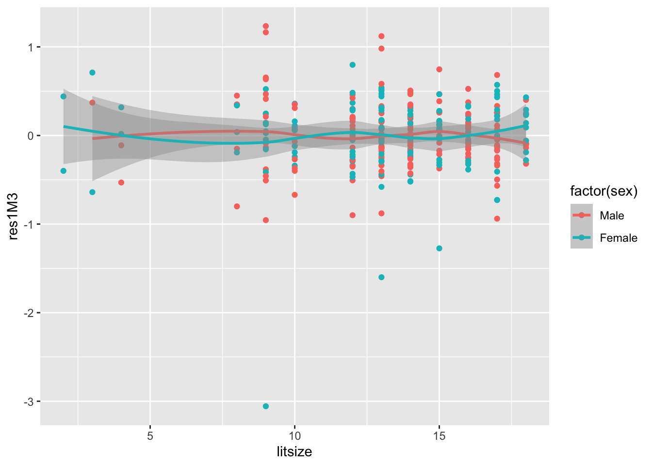 6. (cont.)
a. While some minor patterning is suggested, overall, this does not seem like a non-linear effect has been omitted, nor is there strong evidence of heteroscedasticity.
- If we wanted to look at treatment X littersize interactions, these would be entered on level 2:
Code
## Linear mixed model fit by REML. t-tests use Satterthwaite's method ['lmerModLmerTest']
## Formula: weight ~ treatment + litsize + factor(treatment):litsize + (1 |      litter)
##    Data: ratdat
##
## REML criterion at convergence: 450.3
##
## Scaled residuals:
##     Min      1Q  Median      3Q     Max
## -7.4343 -0.4659 -0.0136  0.5037  3.0826
##
## Random effects:
##  Groups   Name        Variance Std.Dev.
##  litter   (Intercept) 0.07426  0.2725
##  Residual             0.19549  0.4421
## Number of obs: 322, groups:  litter, 27
##
## Fixed effects:
##                               Estimate Std. Error       df t value Pr(>|t|)
## (Intercept)                    8.07191    0.35968 28.72248  22.442  < 2e-16 ***
## treatmentHigh                 -0.30939    0.54000 31.55602  -0.573    0.571
## treatmentLow                  -0.88554    0.54233 37.14040  -1.633    0.111
## litsize                       -0.12220    0.02579 26.76752  -4.738 6.28e-05 ***
## litsize:factor(treatment)High -0.05855    0.04745 29.42653  -1.234    0.227
## litsize:factor(treatment)Low   0.03131    0.03949 34.47790   0.793    0.433
## ---
## Signif. codes:  0 '***' 0.001 '**' 0.01 '*' 0.05 '.' 0.1 ' ' 1
##
## Correlation of Fixed Effects:
##             (Intr) trtmnH trtmnL litsiz lt:()H
## treatmntHgh -0.666
## treatmentLw -0.663  0.442
## litsize     -0.964  0.642  0.639
## ltsz:fct()H  0.524 -0.947 -0.348 -0.544
## ltsz:fct()L 0.630 -0.419 -0.968 -0.653 0.355## Wald test:
## ----------
##
## Chi-squared test:
## X2 = 3.3, df = 2, P(> X2) = 0.2#Pseudo-R2 calculations
- One way to assess the fit of an MLM is through changes in the variance components.
- Singer & Willett suggest using these two measures:
- \(R_W^2 = \frac{{\hat \sigma _\varepsilon ^2({M_0}) - \hat \sigma _\varepsilon ^2({M_1})}}{{\hat \sigma _\varepsilon ^2({M_0})}}\) – this is the proportion reduction in residual (within) variance as we move from model M0 to M1.
- \(R_B^2 = \frac{{\hat \sigma _\zeta ^2({M_0}) - \hat \sigma _\zeta ^2({M_1})}}{{\hat \sigma _\zeta ^2({M_0})}}\) – this is the proportion reduction in between-subject variance as we move from model M0 to M1.
- Clearly this approach works well when the only systematic variation is in the intercept term. 1. It can be used in models with random slopes in one of two ways: ignoring the random slope component, or as a function of the predictors that they modify.
- Referring to the Rat Pup Data, if we compare model M0 to M3:
- \(R_W^2 = \frac{{.20 - .16}}{{.20}} = 0.20\)
- \(R_B^2 = \frac{{.30 - .10}}{{.30}} = 0.67\)
- The within-litter variation was reduced by about 20% with the introduction of the full set of predictors in M3.
- The between-litter variation was reduced by 67% with the introduction of the full set of predictors in M3 – mostly with the introduction of litter size.
- Singer & Willett suggest using these two measures:
#Nested longitudinal series
- Quick introduction to longitudinal data
- Longitudinal (panel) data models involve repeated measurement of the same outcome at different time points.
- Using our nested data modeling framework, we can view those repeated measures as nested within subject.
- The simplest growth curve model could be written: \[ {Y_{ti}} = {b_0} + {\delta_{0i}} + {\varepsilon_{ti}}, \] with \({\delta_{0i}} \sim N(0,\sigma_{{\delta _0}}^2)\) and \({\varepsilon_{ti}} \sim N(0,\sigma _\varepsilon ^2)\). We assume \({\delta_{0i}},\;{\varepsilon_{ti}}\) are independent, throughout.
- (cont.)
- (cont.)
- There is an overall mean for the outcome (here, b0), and it is constant over time. This is the unconditional means model in this setting.
- You should be familiar with this as a random intercept model, with a random intercept for each subject.
- No ‘growth’ is predicted by this model, either at the population (mean) level or individual level.
- This model is clearly misspecified: we expect time to play some role.
- Time can be lots of different things: time since a study began, age, years of schooling, grade level, years on the job, etc. We often represent it with a ‘specially named’ variable, TIME, to reflect this. So the time at occasion t for subject i is TIMEti.
- Under this formulation, TIMEti and occasion ‘t’ are not necessarily the same (think: infant’s age in days).
- Adding time to the basic model for growth, we have: \[ {Y_{ti}} = {b_0} + b_1 TIME_{ti} + {\delta_{0i}} + {\varepsilon_{ti}}, \]
- Time can be lots of different things: time since a study began, age, years of schooling, grade level, years on the job, etc. We often represent it with a ‘specially named’ variable, TIME, to reflect this. So the time at occasion t for subject i is TIMEti.
- (cont.)
with \(\delta_{0i}\sim N(0,\sigma_{\delta_0}^2)\) and \({\varepsilon_{ti}} \sim N(0,\sigma _\varepsilon ^2)\). 1. This is not the unconditional growth model (UGM) described by Singer & Willett; the usual UGM allows individual-specific growth as well.
e. Of course, other covariates can also influence the mean: \[ {Y_{ti}} = {b_0} + {b_1}TIM{E_{ti}} + b_2 X_{2i} + b_3 X_{3ti} + {\delta_{0i}} + {\varepsilon_{ti}} \] 1. (cont.) e. (cont.) i. Here, subscripts on the X terms reflect whether or not they are time-dependent. Those with subscripts ‘ti’ allow for change over time. Those with subscript ‘i’ effectively repeat (in the dataset) for all occasions t. ii. X2 above is constant for each subject (think: race); X3 above can vary over time (think: education). j. Complexity can be added to any of the three components: i. More covariates, interactions or ‘higher order functions of TIME’ (quadratics, cubics) may be added, potentially improving our predictions for the mean, or fixed effects. ii. The systematic variation, \({\delta_{0i}}\) above, can be made more complex (through additional terms and the relationships between them). iii. The residual error structure can also be made more complex. k. We now look at the level or hierarchical form of notation for this type of model. In the top level, we usually limit the covariates to those that either change over time (and thus require reference to both coefficients ‘ti’) or vary at the next ‘level,’ which in this case is the subject-level. So our model is greatly simplified, and can be written:
\[\begin{align*} &\mbox{Level 1: }{Y_{ti}} = {\pi_{0i}} + {\pi_{1i}}TIME_{ti} + {\pi_{2i}}{X_{2ti}} + \varepsilon_{ti} \\ &\mbox{Level 2: } \pi_{0i} = {b_0} + {b_3}{X_{3i}} + \delta_{0i}; \\ &\mbox{\ \ \ \ \ \ \ \ \ \ \ \,} \pi_{1i} = {b_1}; \\ &\mbox{\ \ \ \ \ \ \ \ \ \ \ \,} \pi_{2i} = {b_2}; \\ &\delta_{0i}\sim N(0,\sigma_{\delta_0}^2),\ \varepsilon_{ti}\sim N(0,\sigma_\varepsilon^2), \mbox{ indep.} \end{align*}\]
- (cont.) + The use of \(\pi\) here will eventually make things simpler when we add levels.
- It may seem odd to see X3 as part of the subject-specific constant, but that’s all that a subject-constant predictor can do (a single shift).
- NOTE: we reiterate that we assume normal distributions for the random components: \({\delta_{0i}} \sim N(0,\sigma_{{\delta _0}}^2)\) and \({\varepsilon_{ti}} \sim N(0,\sigma _\varepsilon ^2)\).
- A random slope model is easily added at level 2 as follows:
\[\begin{align*} &\mbox{Level 2: } \pi_{0i} = {b_0} + {b_3}{X_{3i}} + \delta_{0i} \\ &\mbox{\ \ \ \ \ \ \ \ \ \ \ \,} \pi_{1i} = {b_1} + {\delta_{1i}} \\ &\mbox{\ \ \ \ \ \ \ \ \ \ \ \,} \pi_{2i} = {b_2} \\ &\delta_{0i}\sim N(0,\sigma_{\delta_0}^2),\ \delta_{1i} \sim N(0,\sigma_{\delta_1}^2),\ \varepsilon_{ti}\sim N(0,\sigma_\varepsilon^2), \mbox{ indep.} \end{align*}\]
- A common design to study change over time might also involve a nested sampling structure, such as students within classrooms within schools, or individuals within households within buildings within census tracts.
- At the individual level, the subject is tracked over time.
- We have just conceptualized time as another level of grouping, so this type of model is not substantially different from any nested model – except that time has an “elevated” status as a covariate.
- Elevated simply means that it is the first covariate we are likely to consider. Why? Because it is usually a bad idea to leave out a time trend.
- However, to start with a simpler model, we will again leave out the time trend!
- Let us look at an unconditional means model and continue to use level notation. We will introduce an additional level of grouping. Let’s assume a single school, and at first, a sample of classrooms indexed by j within it. We proceed mostly by adding a ‘\(j\)’ to the prior longitudinal model specification (but also note the use of \(\pi\) and \(\beta\)):
\[\begin{align*}
&\mbox{Level 1: }{Y_{tij}} = {\pi_{0ij}} + {\varepsilon_{tij}} \\
&\mbox{Level 2: }\pi_{0ij} = {\beta_{0j}} + {\delta_{0ij}} \\
&\mbox{Level 3: }\beta_{0j} = {b_0} + {\eta_{0j}} \\
&\eta_{0j} \sim N(0,\sigma_{\eta_0}^2),\ \delta_{0ij}\sim N(0,\sigma_{\delta_0}^2), \ \varepsilon_{tij}\sim N(0,\sigma_\varepsilon^2), \mbox{ indep.}
\end{align*}\]
We intentionally leave out the random slope in TIME to keep the model “simple.” You can call \(\eta_{0j},\ \delta_{0ij}, \varepsilon_{tij}\) the level 3,2, and 1 errors, respectively. - You might feel more comfortable with the model in composite notation: \[ {Y_{tij}} = {b_0} + {\delta_{0ij}} + {\eta_{0j}} + {\varepsilon_{tij}} \]
- (cont.)
- Let’s add a time trend. Where does it go? Since time can vary at the individual level, it would go on level 1:
- Let \(TIME_{tij}\) be the time of measurement associated with occasion t on person i in classroom j. TIME could be grade, age, etc.
- Then this model at least contains a fixed effect for TIME: \[ {Y_{tij}} = {b_0} + {b_1}TIME_{tij} + {\delta_{0ij}} + {\eta_{0j}} + {\varepsilon_{tij}} \]
with \({\delta_{0ij}} \sim N(0,\sigma_{{\delta _0}}^2)\), \({\eta_{0j}} \sim N(0,\sigma_{{\eta _0}}^2)\), and \({\varepsilon_{tij}} \sim N(0,\sigma _\varepsilon ^2)\) independently. c. What if we have random slopes (in TIME), say across classrooms: \[ {Y_{tij}} = {b_0} + {b_1}TIME_{tij} + \delta_{0ij} + \eta_{0j} + \eta_{1j}TIME_{tij} + \varepsilon_{tij} \]
with \({\delta_{0ij}} \sim N(0,\sigma_{{\delta _0}}^2)\), \({\eta_{0j}} \sim N(0,\sigma_{{\eta _0}}^2)\), \({\eta_{1j}} \sim N(0,\sigma_{{\eta _1}}^2)\), and \({\varepsilon_{tij}} \sim N(0,\sigma _\varepsilon ^2)\) independently.14
- Adding a new level – schools – should be relatively straightforward: just add a final subscript, k. \[ {Y_{tijk}} = {b_0} + {b_1}TIME_{tijk} + \delta_{0ijk} + \eta_{0jk} + \eta_{1jk}TIME_{tijk} + \zeta_{0k} + \varepsilon_{tijk} \]
with \({\delta_{0ijk}} \sim N(0,\sigma_{{\delta _0}}^2)\), \({\eta_{0jk}} \sim N(0,\sigma_{{\eta _0}}^2)\), \({\eta_{1jk}} \sim N(0,\sigma_{{\eta _1}}^2)\), \({\zeta_{0k}} \sim N(0,\sigma_{{\zeta _0}}^2)\) and \({\varepsilon_{tijk}} \sim N(0,\sigma _\varepsilon ^2)\) independently. b. Another way to understand this model is that we have really just “inserted” a person-specific level shift in the form of \(\delta_{0ijk}\) into our previous model specifications and prepended a subscript ‘\(t\)’ to our indices.
- We now examine several examples of models such as those sketched above.
- We have modified the classroom data to reflect its longitudinal nature. Namely, we have a kindergarten and first grade test score, so we can think of this as a within-subject repeated measure
- It takes slightly complicated code to generate a data frame with a separate entry for each school year from one that contains both, primarily because the names of variables must conform to a specific convention. We then take what is known as a ‘wide’ format to a ‘long’ (or person-period) format as follows:
- We have modified the classroom data to reflect its longitudinal nature. Namely, we have a kindergarten and first grade test score, so we can think of this as a within-subject repeated measure
Code
- (cont.)
- Our baseline model has TIME as the only fixed effect predictor. We include random (intercept, or level) effects for schools and students but not classrooms.
- The random effect for students captures some aspects of the average performance, or level, of each student, net of all else.
- Netting out a student-specific level is similar to controlling for a pre-test, or more accurately, unmeasured, pre-existing abilities or factors.
- Composite notation: \[ MATH_{tijk} = {b_0} + {\delta_{0ijk}} + {\zeta_{0k}} + {b_1}TIM{E_{tijk}} + {\varepsilon_{tijk}}, \]
- The random effect for students captures some aspects of the average performance, or level, of each student, net of all else.
- Our baseline model has TIME as the only fixed effect predictor. We include random (intercept, or level) effects for schools and students but not classrooms.
and we assume \({\delta_{0ijk}} \sim N(0,\sigma_{{\delta_0}}^2)\), \({\zeta_{0k}} \sim N(0,\sigma_{{\zeta_0}}^2)\), and \({\varepsilon_{tijk}} \sim N(0,\sigma _\varepsilon ^2)\). iii. R code and model fit:
## Linear mixed model fit by REML. t-tests use Satterthwaite's method ['lmerModLmerTest']
## Formula: math ~ year + (1 | schoolid/childid)
## Data: class_pp
##
## REML criterion at convergence: 23554.7
##
## Scaled residuals:
## Min 1Q Median 3Q Max
## -4.7492 -0.4811 0.0085 0.4881 3.4957
##
## Random effects:
## Groups Name Variance Std.Dev.
## childid:schoolid (Intercept) 702.0 26.50
## schoolid (Intercept) 307.5 17.54
## Residual 599.1 24.48
## Number of obs: 2380, groups: childid:schoolid, 1190; schoolid, 107
##
## Fixed effects:
## Estimate Std. Error df t value Pr(>|t|)
## (Intercept) 465.118 2.042 117.023 227.74 <2e-16 ***
## year 57.566 1.003 1189.000 57.37 <2e-16 ***
## ---
## Signif. codes: 0 '***' 0.001 '**' 0.01 '*' 0.05 '.' 0.1 ' ' 1
##
## Correlation of Fixed Effects:
## (Intr)
## year -0.246- (cont.)
- (cont.)
- Comments:
- Math scores are going up, on average, net of school and pupil effects
- The variance components are: \(\sigma_{{\delta_0}}^2 = 702\) (between student, within-school variation); \(\sigma_{{\zeta _0}}^2 = 308\) (between-school variation for the average student in each school); \(\sigma _\varepsilon ^2 = 599\) (within-school, within-student variation; this is variation over time).
- Notice the slightly different way we frame these effects in this context.
- Notice that uncertainty within student is as large as between.
- Comments:
- (cont.)
- Our next model adds a random intercept for classrooms, to see if it is ‘needed.’
- Composite notation: \[ MATH_{tijk} = {b_0} + {\delta_{0ijk}} + {\eta_{0jk}} + {\zeta_{0k}} + {b_1}TIME_{tijk} + {\varepsilon_{tijk}} \]
and assume \({\delta_{0ijk}} \sim N(0,\sigma_{{\delta_0}}^2)\), \({\eta_{0jk}} \sim N(0,\sigma_{{\eta_{00}}}^2)\), \({\zeta_{0k}} \sim N(0,\sigma_{{\zeta_0}}^2)\), and \({\varepsilon_{tijk}} \sim N(0,\sigma _\varepsilon ^2)\), independently. iii. R code and model fit (with a preliminary comment). 1. This is the first time we have three levels of nesting, so it is worth examining the nested structure closely.
Code
fit.M0 <- lmer(math~year+(1|schoolid)+(1|schoolid:classid)+(1|classid:childid),data=class_pp) #shortcut to get model to fit in reasonable amount of time.
#alternative:
fit.M0 <- lmer(math~year+(1|schoolid/classid/childid),data=class_pp) #shortcut to get model to fit in reasonable amount of time.
print(summary(fit.M0))## Linear mixed model fit by REML. t-tests use Satterthwaite's method ['lmerModLmerTest']
## Formula: math ~ year + (1 | schoolid/classid/childid)
## Data: class_pp
##
## REML criterion at convergence: 23552.8
##
## Scaled residuals:
## Min 1Q Median 3Q Max
## -4.7533 -0.4887 0.0124 0.4941 3.4835
##
## Random effects:
## Groups Name Variance Std.Dev.
## childid:(classid:schoolid) (Intercept) 675.98 26.000
## classid:schoolid (Intercept) 39.01 6.246
## schoolid (Intercept) 294.31 17.156
## Residual 599.05 24.476
## Number of obs: 2380, groups:
## childid:(classid:schoolid), 1190; classid:schoolid, 312; schoolid, 107
##
## Fixed effects:
## Estimate Std. Error df t value Pr(>|t|)
## (Intercept) 465.062 2.045 117.683 227.46 <2e-16 ***
## year 57.566 1.003 1189.005 57.37 <2e-16 ***
## ---
## Signif. codes: 0 '***' 0.001 '**' 0.01 '*' 0.05 '.' 0.1 ' ' 1
##
## Correlation of Fixed Effects:
## (Intr)
## year -0.245## Data: class_pp
## Models:
## fit.M00: math ~ year + (1 | schoolid/childid)
## fit.M0: math ~ year + (1 | schoolid/classid/childid)
## npar AIC BIC logLik deviance Chisq Df Pr(>Chisq)
## fit.M00 5 23565 23594 -11777 23555
## fit.M0 6 23565 23599 -11776 23553 1.8954 1 0.1686- (cont.)
- The LR test is non-significant. 1. However, we will leave in classroom effects for discussion purposes.
- Ask yourself: is there enough information in the data to estimate all of the parameters in this model? \(\sigma^2_{\delta_0}\) in particular is the most challenging. Would you be able to estimate a random slope in time at the person-level? Maybe; think about degrees of freedom.
- Our next model adds a random slope effect (in TIME) for schools. This is closer to what Singer & Willett call an unconditional growth model: we have differences (at the school level) in how those trajectories change over time…or do we?
- Composite notation: \[ MATH_{tijk} = {b_0} + {\delta_{0ijk}} + {\eta_{0jk}} + {\zeta_{0k}} + ({b_1} + {\zeta_{1k}})TIM{E_{tijk}} + {\varepsilon_{tijk}} \]
and assume \({\delta_{0ijk}} \sim N(0,\sigma_{{\delta _0}}^2)\), \({\eta_{0jk}} \sim N(0,\sigma_{{\eta _0}}^2)\), \({\zeta_{0k}} \sim N(0,\sigma_{{\zeta _0}}^2)\), \({\zeta_{1k}} \sim N(0,\sigma_{{\zeta _1}}^2)\) and \({\varepsilon_{tijk}} \sim N(0,\sigma _\varepsilon ^2)\). iii. STATA code and model fit:
Code
## Linear mixed model fit by REML. t-tests use Satterthwaite's method ['lmerModLmerTest']
## Formula: math ~ year + (year || schoolid) + (1 | schoolid:classid) + (1 | classid:childid)
## Data: class_pp
##
## REML criterion at convergence: 23527.2
##
## Scaled residuals:
## Min 1Q Median 3Q Max
## -4.7699 -0.4749 0.0113 0.4644 3.5957
##
## Random effects:
## Groups Name Variance Std.Dev.
## classid.childid (Intercept) 699.50 26.448
## schoolid.classid (Intercept) 38.33 6.191
## schoolid year 88.57 9.411
## schoolid.1 (Intercept) 312.12 17.667
## Residual 552.23 23.499
## Number of obs: 2380, groups: classid:childid, 1190; schoolid:classid, 312; schoolid, 107
##
## Fixed effects:
## Estimate Std. Error df t value Pr(>|t|)
## (Intercept) 465.028 2.084 110.506 223.12 <2e-16 ***
## year 57.501 1.370 99.876 41.98 <2e-16 ***
## ---
## Signif. codes: 0 '***' 0.001 '**' 0.01 '*' 0.05 '.' 0.1 ' ' 1
##
## Correlation of Fixed Effects:
## (Intr)
## year -0.177## Data: class_pp
## Models:
## fit.M0: math ~ year + (1 | schoolid/classid/childid)
## fit.M1: math ~ year + (year || schoolid) + (1 | schoolid:classid) + (1 | classid:childid)
## npar AIC BIC logLik deviance Chisq Df Pr(>Chisq)
## fit.M0 6 23565 23599 -11776 23553
## fit.M1 7 23541 23582 -11764 23527 25.52 1 4.377e-07 ***
## ---
## Signif. codes: 0 '***' 0.001 '**' 0.01 '*' 0.05 '.' 0.1 ' ' 1- (cont.)
- We have evidence from the LRT that random slopes add explanatory power (test of H0: \(\sigma_{{\zeta _1}}^2 = 0\)):
- The ‘new’ variance components are: \(\sigma_{{\zeta _0}}^2 = 312\) and \(\sigma_{{\zeta _1}}^2 = 89\).
- The corresponding school-level effects enter the model in these two terms: \({\zeta_{0k}} + {\zeta_{1k}}TIM{E_{tijk}}\).
- This translates into two different between-school variances (call this a function, VB-S(t)), one at time 0 and one at time 1:
- \({V_{B - S}}(0) = \sigma_{{\zeta _0}}^2 + 0 \cdot \sigma_{{\zeta _1}}^2 = 312\)
- \({V_{B - S}}(1) = \sigma_{{\zeta _0}}^2 + {1^2} \cdot \sigma_{{\zeta _1}}^2 = 312 + 89 = 401\)
We will eventually check whether the variance between schools is statistically larger in first grade. It’s important to be aware of how heteroscedasticity is implicitly included in a model this way, through the random slope terms.
- Our next model moves the random slope effect (in TIME) to classrooms – a much smaller unit on which to base estimation. Again, we examine whether we have differences (at the classroom level) in how those trajectories change over time.
- Composite notation: \[ MATH_{tijk} = {b_0} + {\delta_{0ijk}} + {\eta_{0jk}} + {\zeta_{0k}} + ({b_1} + {\eta_{1jk}})TIM{E_{tijk}} + \varepsilon_{tijk} \]
- For both notations, we assume \({\delta_{0ijk}} \sim N(0,\sigma_{{\delta _0}}^2)\), \({\eta_{0jk}} \sim N(0,\sigma_{{\eta _0}}^2)\), \({\eta_{1jk}} \sim N(0,\sigma_{{\eta _1}}^2)\), \({\zeta_{0k}} \sim N(0,\sigma_{{\zeta _0}}^2)\) and \({\varepsilon_{tijk}} \sim N(0,\sigma _\varepsilon ^2)\).
- STATA code and model fit:
Code
## Linear mixed model fit by REML. t-tests use Satterthwaite's method ['lmerModLmerTest']
## Formula: math ~ year + (1 | schoolid) + (year || schoolid:classid) + (1 | classid:childid)
## Data: class_pp
##
## REML criterion at convergence: 23530.8
##
## Scaled residuals:
## Min 1Q Median 3Q Max
## -4.7720 -0.4608 0.0021 0.4687 3.6375
##
## Random effects:
## Groups Name Variance Std.Dev.
## classid.childid (Intercept) 710.07 26.647
## schoolid.classid year 117.47 10.838
## schoolid.classid.1 (Intercept) 21.57 4.644
## schoolid (Intercept) 310.69 17.626
## Residual 534.75 23.125
## Number of obs: 2380, groups: classid:childid, 1190; schoolid:classid, 312; schoolid, 107
##
## Fixed effects:
## Estimate Std. Error df t value Pr(>|t|)
## (Intercept) 465.112 2.062 111.926 225.58 <2e-16 ***
## year 57.311 1.162 313.622 49.33 <2e-16 ***
## ---
## Signif. codes: 0 '***' 0.001 '**' 0.01 '*' 0.05 '.' 0.1 ' ' 1
##
## Correlation of Fixed Effects:
## (Intr)
## year -0.192## Data: class_pp
## Models:
## fit.M0: math ~ year + (1 | schoolid/classid/childid)
## fit.M2: math ~ year + (1 | schoolid) + (year || schoolid:classid) + (1 | classid:childid)
## npar AIC BIC logLik deviance Chisq Df Pr(>Chisq)
## fit.M0 6 23565 23599 -11776 23553
## fit.M2 7 23545 23585 -11765 23531 21.956 1 2.789e-06 ***
## ---
## Signif. codes: 0 '***' 0.001 '**' 0.01 '*' 0.05 '.' 0.1 ' ' 1- (cont.)
- LRT suggests that random slopes for classrooms are needed (when they have been omitted at the school level):
- The classroom-based variance components are: \(\sigma_{{\eta _0}}^2 = 22\) and \(\sigma_{{\eta _1}}^2 = 117\).
- The corresponding classroom-level effects enter the model in these two terms: \({\eta_{0jk}} + {\eta_{1jk}}TIM{E_{tijk}}\).
- This translates into two different between-classroom variances (VB-C(t)):
- \({V_{B - C}}(0) = \sigma_{{\eta _0}}^2 + 0 \cdot \sigma_{{\eta _1}}^2 = 22\)
- \({V_{B - C}}(1) = \sigma_{{\eta _0}}^2 + 1 \cdot \sigma_{{\eta _1}}^2 = 22 + 117 = 139\)
- This dramatic difference between the two grade levels really should (and will) be tested formally.
- A graph can be made of V(t) or V(X), any X.
- Our next model contains a random slope effect (in TIME) for both classrooms and schools. Again, we examine whether we have differences (at both levels) in how those trajectories change over time.
- Composite notation: \[ MATH_{tijk} = {b_0} + {\delta_{0ijk}} + {\eta_{0jk}} + {\zeta_{0k}} + ({b_1} + {\eta_{1jk}} + {\zeta_{1k}})TIM{E_{tijk}} + {\varepsilon_{tijk}} \] assume \({\delta_{0ijk}} \sim N(0,\sigma_{{\delta_0}}^2)\), \({\eta_{0jk}} \sim N(0,\sigma_{{\eta_0}}^2)\), \({\eta_{1jk}} \sim N(0,\sigma_{{\eta_1}}^2)\), \({\zeta_{0k}} \sim N(0,\sigma_{{\zeta_0}}^2)\), \({\zeta_{1k}} \sim N(0,\sigma_{{\zeta_1}}^2)\) and \({\varepsilon_{tijk}} \sim N(0,\sigma _\varepsilon ^2)\).
- R code and model fit:
Code
## Linear mixed model fit by REML. t-tests use Satterthwaite's method ['lmerModLmerTest']
## Formula: math ~ year + (year || schoolid/classid) + (1 | classid:childid)
## Data: class_pp
##
## REML criterion at convergence: 23521.7
##
## Scaled residuals:
## Min 1Q Median 3Q Max
## -4.7783 -0.4702 0.0115 0.4617 3.6485
##
## Random effects:
## Groups Name Variance Std.Dev.
## classid.childid (Intercept) 711.99 26.683
## classid.schoolid year 60.92 7.805
## classid.schoolid.1 (Intercept) 25.32 5.032
## schoolid year 69.36 8.328
## schoolid.1 (Intercept) 318.69 17.852
## Residual 529.96 23.021
## Number of obs: 2380, groups: classid:childid, 1190; classid:schoolid, 312; schoolid, 107
##
## Fixed effects:
## Estimate Std. Error df t value Pr(>|t|)
## (Intercept) 465.071 2.085 109.673 223.08 <2e-16 ***
## year 57.349 1.371 98.610 41.83 <2e-16 ***
## ---
## Signif. codes: 0 '***' 0.001 '**' 0.01 '*' 0.05 '.' 0.1 ' ' 1
##
## Correlation of Fixed Effects:
## (Intr)
## year -0.169The variance components generate a fair amount of heteroscedasticity. The significance of the random slope terms is confirmed through these two LRTs:
## Data: class_pp
## Models:
## fit.M1: math ~ year + (year || schoolid) + (1 | schoolid:classid) + (1 | classid:childid)
## fit.M3: math ~ year + (year || schoolid/classid) + (1 | classid:childid)
## npar AIC BIC logLik deviance Chisq Df Pr(>Chisq)
## fit.M1 7 23541 23582 -11764 23527
## fit.M3 8 23538 23584 -11761 23522 5.5304 1 0.01869 *
## ---
## Signif. codes: 0 '***' 0.001 '**' 0.01 '*' 0.05 '.' 0.1 ' ' 1## Data: class_pp
## Models:
## fit.M2: math ~ year + (1 | schoolid) + (year || schoolid:classid) + (1 | classid:childid)
## fit.M3: math ~ year + (year || schoolid/classid) + (1 | classid:childid)
## npar AIC BIC logLik deviance Chisq Df Pr(>Chisq)
## fit.M2 7 23545 23585 -11765 23531
## fit.M3 8 23538 23584 -11761 23522 9.0945 1 0.002564 **
## ---
## Signif. codes: 0 '***' 0.001 '**' 0.01 '*' 0.05 '.' 0.1 ' ' 1NOTE: You should be able to state what the assumptions are (the base model) and what the null hypothesis is (whatever is added has coefficients equal to zero) in both LRTs, above.
Importantly, we do not know, from the above tests, whether each of the random intercepts is still needed.
In particular, it seems unlikely that the random intercept for classrooms is needed, once the same is included for schools. We can test this formally by fitting yet another model:
Code
## Linear mixed model fit by REML. t-tests use Satterthwaite's method ['lmerModLmerTest']
## Formula: math ~ year + (year || schoolid) + (0 + year | schoolid:classid) +
## (1 | classid:childid)
## Data: class_pp
##
## REML criterion at convergence: 23522.4
##
## Scaled residuals:
## Min 1Q Median 3Q Max
## -4.7799 -0.4658 0.0112 0.4606 3.6624
##
## Random effects:
## Groups Name Variance Std.Dev.
## classid.childid (Intercept) 727.57 26.974
## schoolid.classid year 64.17 8.011
## schoolid year 68.43 8.272
## schoolid.1 (Intercept) 327.61 18.100
## Residual 529.30 23.006
## Number of obs: 2380, groups: classid:childid, 1190; schoolid:classid, 312; schoolid, 107
##
## Fixed effects:
## Estimate Std. Error df t value Pr(>|t|)
## (Intercept) 465.102 2.084 109.253 223.22 <2e-16 ***
## year 57.338 1.371 98.538 41.81 <2e-16 ***
## ---
## Signif. codes: 0 '***' 0.001 '**' 0.01 '*' 0.05 '.' 0.1 ' ' 1
##
## Correlation of Fixed Effects:
## (Intr)
## year -0.168## Data: class_pp
## Models:
## fit.MM3: math ~ year + (year || schoolid) + (0 + year | schoolid:classid) + (1 | classid:childid)
## fit.M3: math ~ year + (year || schoolid/classid) + (1 | classid:childid)
## npar AIC BIC logLik deviance Chisq Df Pr(>Chisq)
## fit.MM3 7 23536 23577 -11761 23522
## fit.M3 8 23538 23584 -11761 23522 0.7306 1 0.3927It seems we do not need the level effects for classrooms (so school level intercept suffices), with school effects in the model, but the random slopes are still useful at the classroom level. We have not tested the last point formally, but we can expect the likelihood to essentially be unchanged with the random classroom intercept dropped; under this scenario, the prior LRT that examined the ‘need’ for random classroom slopes should prevail.
- One last thing to explore is whether our models for heteroscedasticity are consistent with prior findings.
- These models assign greater variation at the classroom or school level to first grade math scores.
- We check this by reloading the original data (wide format) and running some simple models (child-level effects cannot enter into models such as these as there is no replication at that level):
Code
## Linear mixed model fit by REML. t-tests use Satterthwaite's method ['lmerModLmerTest']
## Formula: mathkind ~ 1 + (1 | schoolid/classid)
## Data: dat
##
## REML criterion at convergence: 12085.1
##
## Scaled residuals:
## Min 1Q Median 3Q Max
## -4.8198 -0.5749 0.0012 0.6303 3.5893
##
## Random effects:
## Groups Name Variance Std.Dev.
## classid:schoolid (Intercept) 32.0 5.657
## schoolid (Intercept) 352.8 18.784
## Residual 1323.4 36.379
## Number of obs: 1190, groups: classid:schoolid, 312; schoolid, 107
##
## Fixed effects:
## Estimate Std. Error df t value Pr(>|t|)
## (Intercept) 465.220 2.191 103.579 212.4 <2e-16 ***
## ---
## Signif. codes: 0 '***' 0.001 '**' 0.01 '*' 0.05 '.' 0.1 ' ' 1Code
## Linear mixed model fit by REML. t-tests use Satterthwaite's method ['lmerModLmerTest']
## Formula: math1st ~ 1 + (1 | schoolid/classid)
## Data: dat
##
## REML criterion at convergence: 11944.6
##
## Scaled residuals:
## Min 1Q Median 3Q Max
## -5.1872 -0.6174 -0.0204 0.5821 3.8339
##
## Random effects:
## Groups Name Variance Std.Dev.
## classid:schoolid (Intercept) 85.46 9.244
## schoolid (Intercept) 280.68 16.754
## Residual 1146.80 33.864
## Number of obs: 1190, groups: classid:schoolid, 312; schoolid, 107
##
## Fixed effects:
## Estimate Std. Error df t value Pr(>|t|)
## (Intercept) 522.540 2.037 104.407 256.6 <2e-16 ***
## ---
## Signif. codes: 0 '***' 0.001 '**' 0.01 '*' 0.05 '.' 0.1 ' ' 1- (cont.)
- The variation at the classroom level follows the basic trend of increasing in first grade, but the effect is muted.
- The variation at the school level drops from kindergarten to first grade, suggesting a misspecification in our nested longitudinal models.
- A reasonable addition is a correlation between the random intercept and slope at the school level in the nested longitudinal data (to leave this out is to potentially misspecify the model):
Code
## Linear mixed model fit by REML. t-tests use Satterthwaite's method ['lmerModLmerTest']
## Formula: math ~ year + (year | schoolid) + (year || schoolid:classid) +
## (1 | classid:childid)
## Data: class_pp
##
## REML criterion at convergence: 23512.8
##
## Scaled residuals:
## Min 1Q Median 3Q Max
## -4.7195 -0.4674 0.0034 0.4598 3.5668
##
## Random effects:
## Groups Name Variance Std.Dev. Corr
## classid.childid (Intercept) 714.68 26.734
## schoolid.classid year 60.44 7.774
## schoolid.classid.1 (Intercept) 25.14 5.014
## schoolid (Intercept) 363.23 19.059
## year 89.36 9.453 -0.50
## Residual 525.06 22.914
## Number of obs: 2380, groups: classid:childid, 1190; schoolid:classid, 312; schoolid, 107
##
## Fixed effects:
## Estimate Std. Error df t value Pr(>|t|)
## (Intercept) 465.081 2.188 103.208 212.59 <2e-16 ***
## year 57.532 1.439 93.791 39.97 <2e-16 ***
## ---
## Signif. codes: 0 '***' 0.001 '**' 0.01 '*' 0.05 '.' 0.1 ' ' 1
##
## Correlation of Fixed Effects:
## (Intr)
## year -0.432## Data: class_pp
## Models:
## fit.M3: math ~ year + (year || schoolid/classid) + (1 | classid:childid)
## fit.M4: math ~ year + (year | schoolid) + (year || schoolid:classid) + (1 | classid:childid)
## npar AIC BIC logLik deviance Chisq Df Pr(>Chisq)
## fit.M3 8 23538 23584 -11761 23522
## fit.M4 9 23531 23583 -11756 23513 8.8936 1 0.002862 **
## ---
## Signif. codes: 0 '***' 0.001 '**' 0.01 '*' 0.05 '.' 0.1 ' ' 1The LRT suggests we ‘need’ the correlation.
- What does this new model imply, in terms of variance between schools at different grades? a. Using the usual formula for variance of a linear combination of (correlated, random) variables, if we have a combination of variables, such as \(X + aY + c\), in which ‘a’ and ‘c’ are constant, but X & Y vary from observation to observation, or group to group, we have, \(Var(X) + 2aCov(X,Y) + {a^2}Var(Y)\) (anything constant that does not multiply something random drops out). b. In our example, the prediction for a school is \[ MATH_{tijk} = {b_0} + {\delta_{0ijk}} + {\eta_{0jk}} + {\zeta_{0k}} + ({b_1} + {\eta_{1jk}} + {\zeta_{1k}})TIME_{tijk} \] but we are focusing on the school-to-school differences, so that everything other than \({\zeta_{0k}} + {\zeta_{1k}}TIME_{tijk}\)behaves like a constant; the expression for variance is \[ {V_{B - S}}(TIME_{tijk}) = \sigma_{{\zeta _0}}^2 + 2TIME_{tijk}\rho_{{\zeta _0}{\zeta _1}} + TIME_{tijk}^2\sigma_{{\zeta _1}}^2 \] yielding: \[ V_{B - S}(0) = \sigma_{{\zeta_0}}^2 + 2 \cdot 0 \cdot {\rho_{{\zeta _0}{\zeta_1}}} + {0^2} \cdot \sigma_{{\zeta_1}}^2 = 363 \] \[ {V_{B - S}}(1) = \sigma_{{\zeta_0}}^2 + 2 \cdot 1 \cdot {\rho_{{\zeta _0}{\zeta_1}}} + {1^2} \cdot \sigma_{{\zeta _1}}^2 = 363 + 2 \cdot ( - 90) + 89 = 272 \]
So the more complex model picks up the ‘drop’ in between-school variance in first grade
5.3 Coding
reshape()is a function to reshape a data frame between wide or long format with repeated measurements. It has arguments as follows:
- data: a data frame
- varying: names of sets of variables in the wide format that correspond to single variables in long format.
- v.name: names of variables in the long format
- timevar: the variable in long format that differentiates multiple records from the same group or individual
- idvar: names of variables in long format that identify multiple records from the same group/individual
- times: the values to use for a newly created timevar variable in long format
- direction: character string to reshape to wide formatCode
# solution
dat <- read.csv("./Datasets/classroom.csv")
#*make a person-period file
dat$math0 <- dat$mathkind
dat$math1 <- dat$mathkind+dat$mathgain
# reshape the data-frame
class_pp <- reshape(dat, varying = c("math0", "math1"),
v.names = "math",
timevar = "year",
times = c(0,1),
direction = "long")
head(class_pp)5.4 Quiz
5.4.1 Self-Assessment
Use “W5 Activity Form” to submit your answers.
- Solve following questions
- 1-A. Run the
ratpupmodels (M0 and M3) defined as below and select the correct R codes for computing the model M0 and M3.
\(\begin{aligned} &\text{Model: M0 } \\ &\text{Level 1: } WEIGHT_{ij} = \beta_{0j} + \epsilon_{ij} \\ &\text{Level 2: } \beta_{0j} = b_{00} + \zeta_{0j} \\ &\varepsilon_{ij}\sim N(0,\sigma_\varepsilon^2), \zeta_{0k}\sim N(0,\sigma_{\zeta_0}^2), independently.\\ \end{aligned}\)
\(\begin{aligned} &\text{Model: M3 } \\ &\text{Level 1: } WEIGHT_{ij} = \beta_{0j} +\beta_{1j}SEX_{ij} \epsilon_{ij} \\ &\text{Level 2: } \beta_{0j} = b_{00} + b_{01}TREAT2_j + b_{02}TREAT3_j + b_{03}LITSIZE_j + \zeta_{0j} \\ & ; \beta_{1j} = b_{10} \\ &\varepsilon_{ij}\sim N(0,\sigma_\varepsilon^2), \zeta_{0k}\sim N(0,\sigma_{\zeta_0}^2), independently.\\ \end{aligned}\)
- 1-B: Write R code to extract the variance components and construct. Report \(R_{W}^2\) and \(R_{B}^2\)
\[\begin{aligned} & R_{W}^2 = \frac{\hat\sigma_{\epsilon}(M_0) - \hat\sigma_{\epsilon}(M_1) }{ \hat\sigma_{\epsilon}(M_0) } \\ & and \\ & R_{B}^2 = \frac{\hat\sigma_{\zeta}(M_0) - \hat\sigma_{\zeta}(M_1) }{ \hat\sigma_{\zeta}(M_0) } \end{aligned}\]
- 1-C: With this experimental design, which type of variation (between or within litter) is expected to be explained by the treatment? Why?
- Solve following questions
- 2-A: Fit these models for Nested Longitudinal Data as below and select the correct R codes for computing the model M1 and M2.
\[\begin{aligned} &\text{M1: } Y_{tijk} = b_0 + b_1TIME_{tijk} + \delta_{0ijk} + \eta_{0jk} + \zeta_{0k} + \epsilon_{tijk} \\ &\text{M2: } Y_{tijk} = b_0 + b_1TIME_{tijk} + \delta_{0ijk} + \eta_{0jk} + \eta_{1jk}TIME_{tijk} + \zeta_{0k} + \epsilon_{tijk} \\ \end{aligned}\]
2-B: Calculate \(V_{BC}\) which does not depend on grade
2-C: Calculate \(V_{BC}(0)\), \(V_{BC}(1)\) which is a between classroom variance at grade 0 followed by grade 1
2-D: Why are there a (0) and (1) as inputs to the variance ‘function’?
2-E: Why is this an example of heteroscedasticity? Give as much detail as you can.
2-F: Explain why the dramatic difference is a concern, given the prior models that were fit?
2-G: Run separate models and report separately, \(V_{BC}(0), V_{BC}(1).\)
2-H: Explain how running separate models (in the notes) allows us to find flaws in the original model’s fit.
Code
# solution
require(lme4)
require(lmerTest)
require(aod)
ratdat <- read.table("./Datasets/rat_pup.dat",header=T)
fit.M0 <- lmer(weight~1+(1|litter),data=ratdat)
ratdat$sex <- factor(ratdat$sex,levels=c("Male","Female"))
fit.M3 <- lmer(weight~factor(treatment)+factor(sex)+litsize+(1|litter),data=ratdat)
Sig2.M0.between <- attr(VarCorr(fit.M0)[["litter"]],"stddev")^2
Sig2.M0.within <- summary(fit.M0)$sigma^2
Sig2.M3.between <- attr(VarCorr(fit.M3)[["litter"]],"stddev")^2
Sig2.M3.within <- summary(fit.M3)$sigma^2
R2.W <- (Sig2.M0.within-Sig2.M3.within)/Sig2.M0.within
R2.B <- (Sig2.M0.between-Sig2.M3.between)/Sig2.M0.between
paste(R2.W)## [1] "0.170680940747386"## [1] "0.675734118926159"Code
# solution
dat <- read.csv("./Datasets/classroom.csv")
#*make a person-period file
dat$math0 <- dat$mathkind
dat$math1 <- dat$mathkind+dat$mathgain
class_pp <- reshape(dat,varying = c("math0", "math1"),v.names = "math",timevar = "year",times = c(0,1),direction = "long")
fit.M1 <- lmer(math ~ year + (1 | schoolid) + (1|schoolid:classid) + (1|classid:childid), data=class_pp)
fit.M2 <- lmer(math ~ year + (1 | schoolid) + (year || schoolid:classid) + (1|classid:childid), data=class_pp)5.4.2 Lab Quiz
- Review the material in the Rshiny app “Week5: Handout5 Activity” and then answer these questions on the google form “W5 Activity Form”
5.4.3 Homework
- Homework is presented as the last section of the Rshiny app “Week5: Handout5 Activity”.
- Follow instructions there (fill out this form “W5 Activity Form” ) and hand in your code on Brightspace