Chapter 6 : Centering; ecological fallacy; hybrid model; FE v. RE
Code
vanillaR <- F
showR <- T
liveDemo <- F
library(ggplot2)
require(foreign)
require(lme4)
library(lmerTest)
library(plm)#for hausman test
library(aod)#for wald test
#insheet using "classroom.csv", comma clear
dat <- read.csv("./Datasets/classroom.csv")
if(!require(plm)) install.packages(plm)
library(plm)
6.1 Centering
- Centering
- Grand mean: In MLMs, centering on a grand mean is not that different than what is commonly done in regression. You simply shift the “zero” or origin of the predictor.
- This shifts the ‘reference group’ to the average of any predictor you have grand mean centered, which could be useful.
- This is more useful as an anchor than you might imagine. E.g., when you wish to compare the constant across nested models, the reference group never changes.
- Centering can reduce multicollinearity that is common among interactions, especially squared and higher order terms.
- This shifts the ‘reference group’ to the average of any predictor you have grand mean centered, which could be useful.
- Group-mean centering, however, has the potential to change all of your estimates.
- Group-mean centering entails computing the mean for a predictor separately for each group and then subtracting out those group-specific means before entering that predictor in the model.
- They become relative effects: what does a one unit change from my group average lead to in terms of the outcome, net of all else?
- The two effects are potentially quite different, as will become immediately apparent from our simulated data. We generate our data using this ‘model’:
- Grand mean: In MLMs, centering on a grand mean is not that different than what is commonly done in regression. You simply shift the “zero” or origin of the predictor.
\[ {y_{ij}} = 1 \cdot {x_{ij}} + {\eta_j} + {\varepsilon_{ij}} \] \[ {x_{ij}} = j + {\upsilon_{ij}} \] \[ \mbox{with }{\eta_j} = 1.1 \cdot (31 - j),\ j = 1 \ldots 30 \] \[ \varepsilon_{ij}\sim N(0,{0.5^2}),\ {\upsilon_{ij}} \sim N(0,{1^2}) \mbox{ indep.} \] This implies that group 1 has an effect (\(\eta\)) of 1.1x30; group 2 has an effect of 1.1x29; …; group 30 has an effect of 1.1x1. 1. By assigning group effects that are decreasing as group number (and ‘x’) increases, we generate two ‘conflicting’ relationships (within vs. between). iv. Below, we plot outcome ‘y’ by predictor ‘x’, when the data are grouped (by color), which reveals the difference between the two effects:
Code
require(foreign)
require(nlme)
set.seed(2042)
M <- 10 # obs per group
K <- 30 # groups
id <- rep(1:K,rep(M,K))
x <- rnorm(M*K)+ id
m <- 1.1
y <- 1*x + rnorm(M*K,sd=.5) + rep(seq(m*K,m,-m),each=M)
#this more 'normal' eta leads to LMEs doing 'better'
#y <- 1*x + rnorm(M*K,sd=.5) + 1.5*rep(m*K*(1.96+qnorm(seq(.975,0.025,length=K)))/3.92,each=M)

ggplot(data=NULL,aes(x=x,y=y,col=id)) +
  geom_point() +
  scale_color_gradientn(colours = rainbow(K)) +
  theme_classic()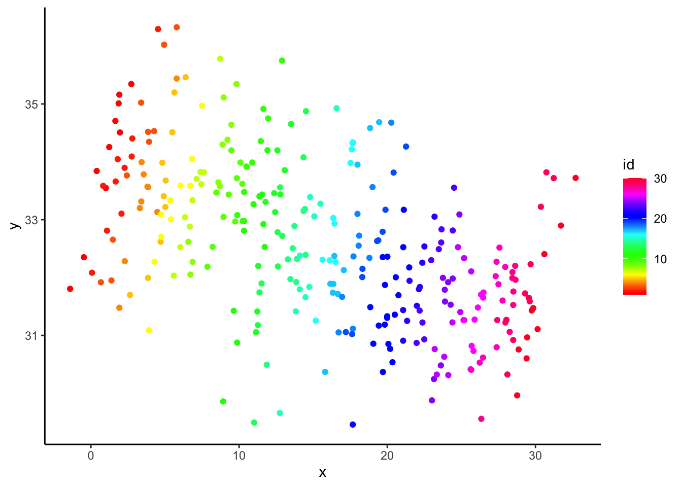
- (cont.)
- (cont.)
- Can you see the ‘conflict’? Within group, there is a positive relationship, and between, there is a negative one.
- This is an example of the ecological fallacy: the relationship in the aggregate differs from the relationship at the individual level.
- Simple OLS regression (G&H’s “Completely Pooled” approach) picks up the overall, negative slope:
- Can you see the ‘conflict’? Within group, there is a positive relationship, and between, there is a negative one.
- (cont.)
##
## Call:
## lm(formula = y ~ x)
##
## Residuals:
##     Min      1Q  Median      3Q     Max
## -3.4506 -0.7961  0.0034  0.6415  2.9588
##
## Coefficients:
##              Estimate Std. Error t value Pr(>|t|)
## (Intercept) 33.840126   0.138874  243.68   <2e-16 ***
## x           -0.081299   0.007807  -10.41   <2e-16 ***
## ---
## Signif. codes:  0 '***' 0.001 '**' 0.01 '*' 0.05 '.' 0.1 ' ' 1
##
## Residual standard error: 1.18 on 298 degrees of freedom
## Multiple R-squared:  0.2668, Adjusted R-squared:  0.2644
## F-statistic: 108.5 on 1 and 298 DF, p-value: < 2.2e-16- (cont.)
- (cont.)
- Random intercept MLMs don’t help us (much) in this instance:
- (cont.)
## Linear mixed-effects model fit by REML
##   Data: NULL
##
## Random effects:
##  Formula: ~1 | id
##         (Intercept) Residual
## StdDev:   0.3193014 1.141441
##
## Fixed effects:  y ~ x
##  Correlation:
##   (Intr)
## x -0.871
##
## Standardized Within-Group Residuals:
##         Min          Q1         Med          Q3         Max
## -2.85230865 -0.66624251 -0.02169386  0.56618706  2.47012199
##
## Number of Observations: 300
## Number of Groups: 30- (cont.)
- (cont.)
- (cont.)
- Random effects MLMs actually estimate the single effect for ‘x’ as a mixture of between (completely pooled) and within (unpooled, mini-regressions, one for each group) group effects.
- The mixing weights depend in part on the ICC.
- The smaller ICC in this example may be part of the ‘problem,’ but it isn’t that simple.
- Our simulation used ‘effects’ that were uniform - not normal – this could be a part of the problem as well.
- Random effects MLMs actually estimate the single effect for ‘x’ as a mixture of between (completely pooled) and within (unpooled, mini-regressions, one for each group) group effects.
- Group-mean centering will pick up the within-group relationship.
- (cont.)
- Some details about group-mean centering (CWC; center within cluster, Enders & Tofighi terminology)
- Here, we build intuition for what group-mean centering is ‘doing’
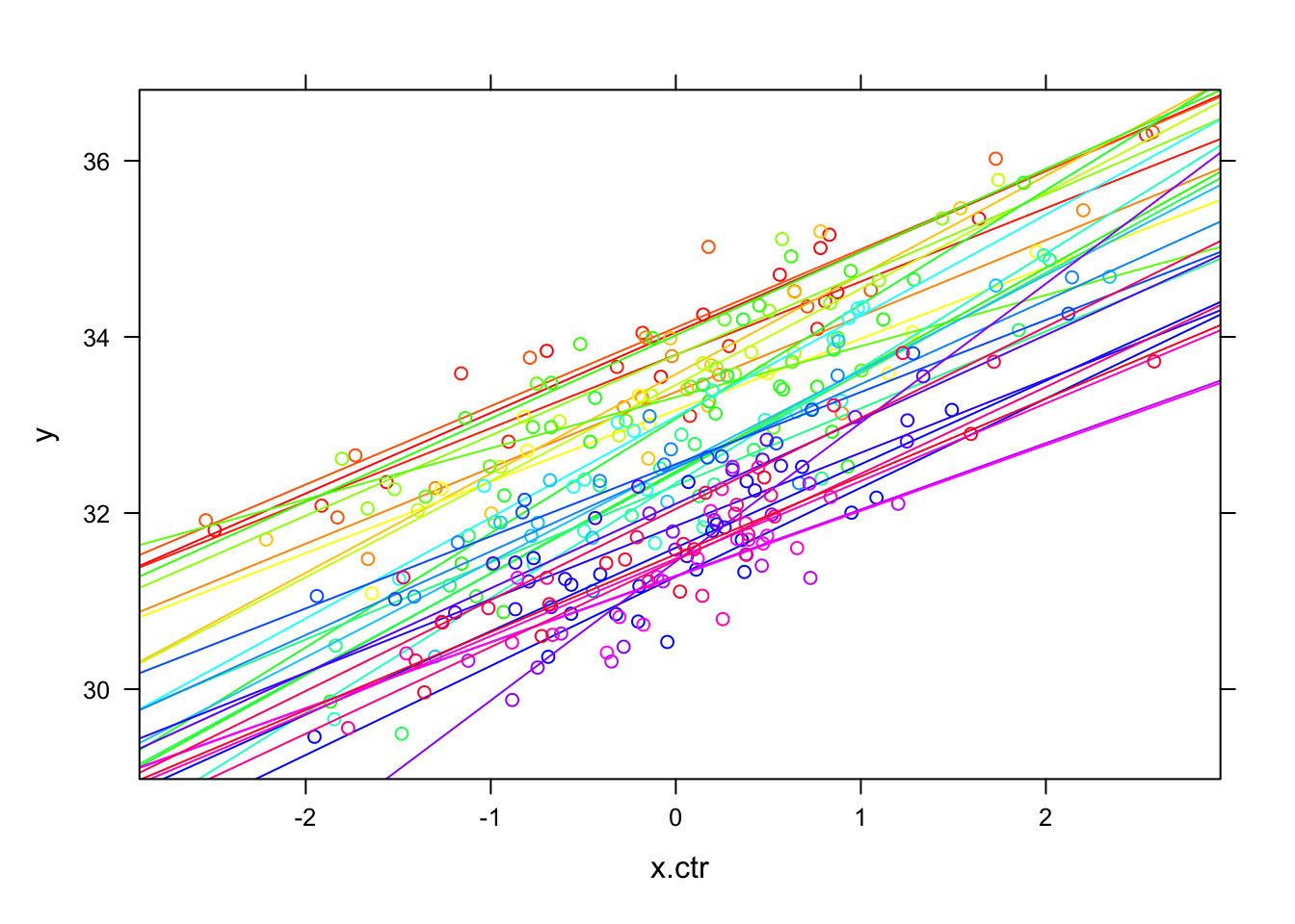
- When viewed separately for each group ID, the effect is clearly strong and positive:
- (cont.)
Code
## `geom_smooth()` using formula = 'y ~ x'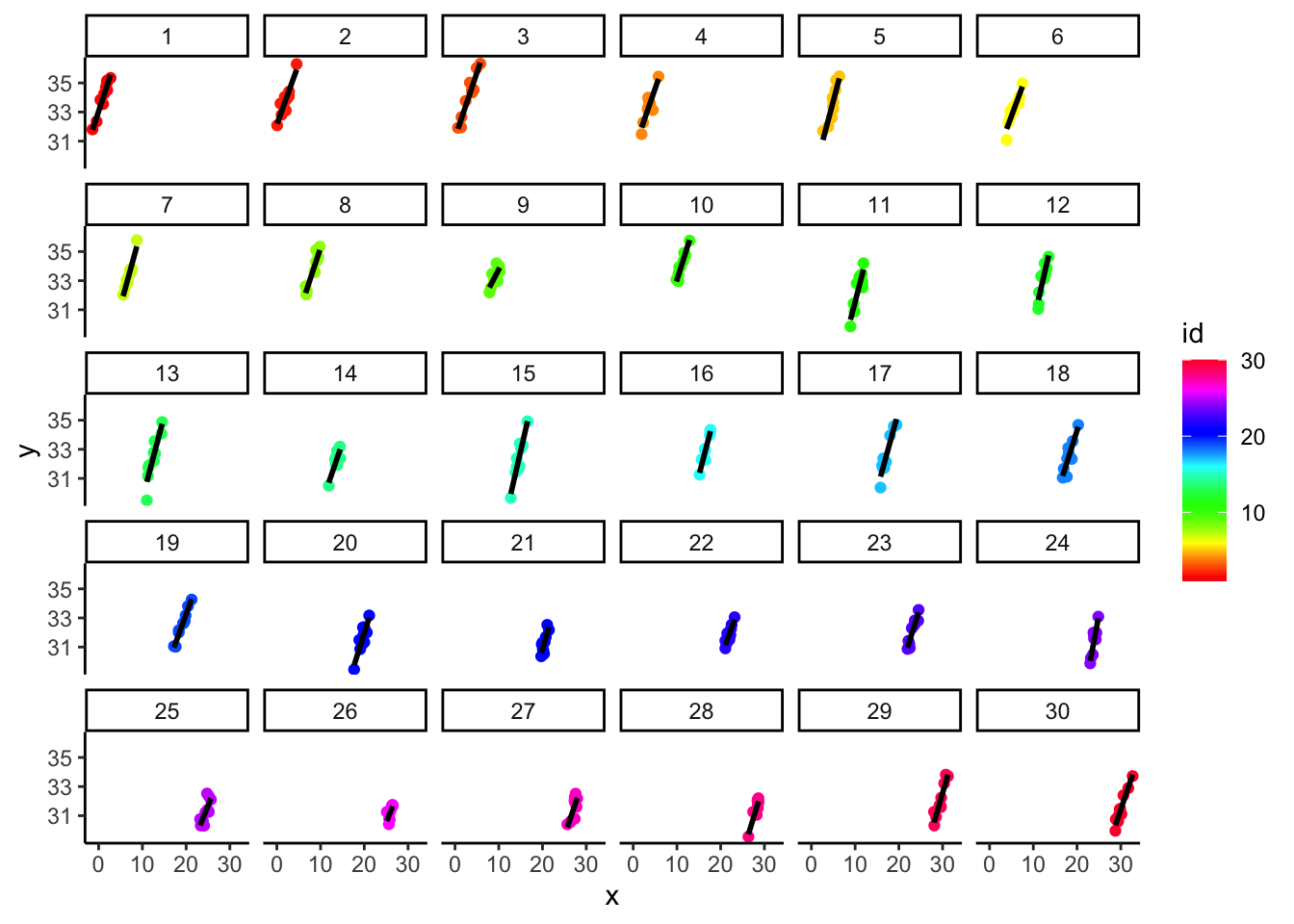
- (cont.)
- (cont.)
- But when viewed in the aggregate, you can see it would be hard to model the within-group relationships separately from the between-group ones.
1. In fact, CWC allows one to model each relationship separately.
2. The plot, below, reveals the two distinct relationships
- Actually the negative relationship (in grey, below) is slightly different from the effect based on the regression of outcome-group-means on predictor-group-means, but it is very nearly the same (and easier to include in the ‘statistical programming’).
- But when viewed in the aggregate, you can see it would be hard to model the within-group relationships separately from the between-group ones.
1. In fact, CWC allows one to model each relationship separately.
2. The plot, below, reveals the two distinct relationships
- (cont.)
Code
## `geom_smooth()` using formula = 'y ~ x'
## `geom_smooth()` using formula = 'y ~ x'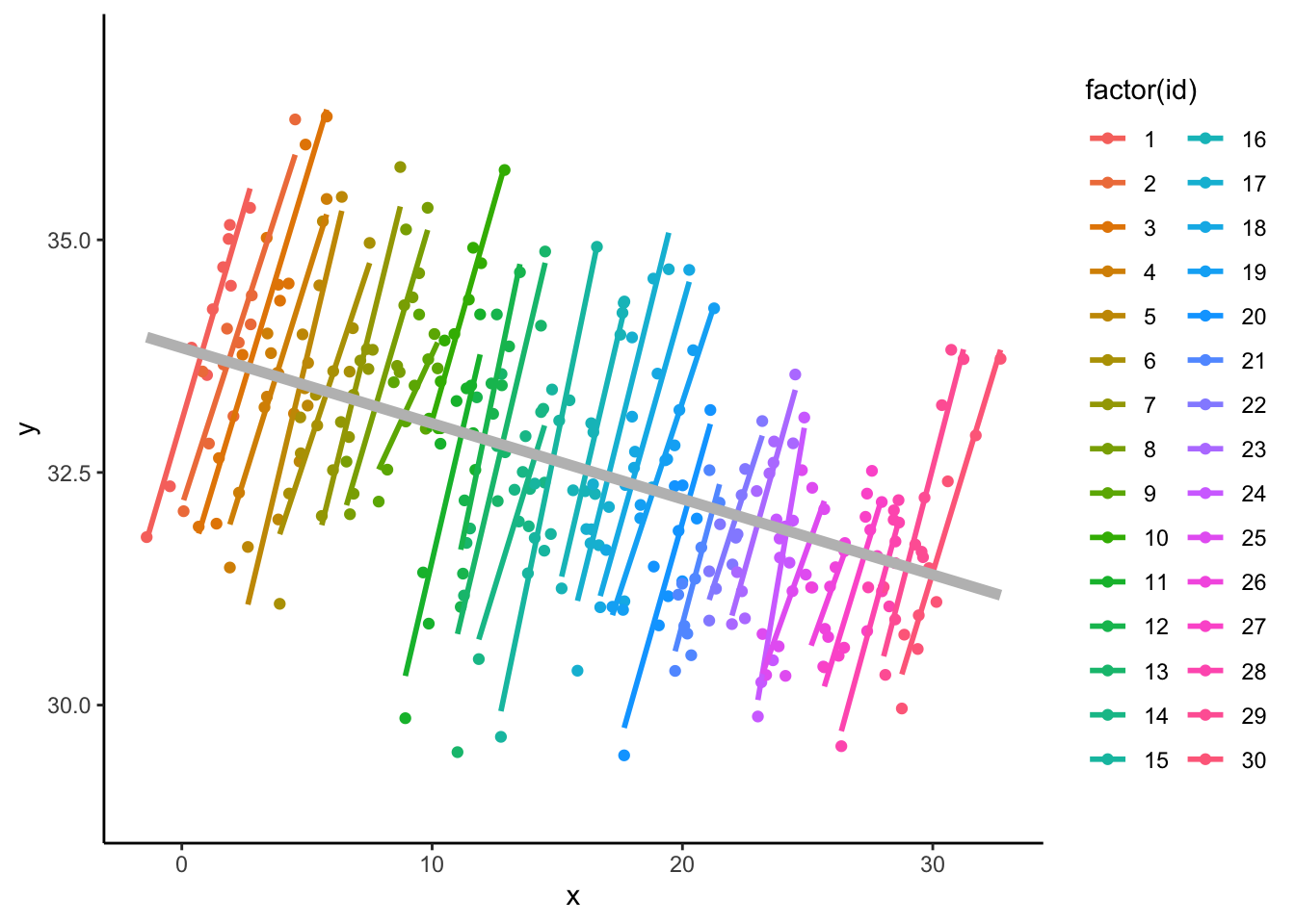
- (cont.)
- (cont.)
- The exact relationship of the group means is about -0.1, as this group-level analysis, below, reveals:
- (cont.)
Code
##
## Call:
## lm(formula = mn.y ~ mn.x)
##
## Residuals:
##      Min       1Q   Median       3Q      Max
## -0.84234 -0.33638  0.03483  0.23102  1.01617
##
## Coefficients:
##              Estimate Std. Error t value Pr(>|t|)
## (Intercept) 34.039671   0.163393  208.33  < 2e-16 ***
## mn.x        -0.094170   0.009198  -10.24 5.72e-11 ***
## ---
## Signif. codes:  0 '***' 0.001 '**' 0.01 '*' 0.05 '.' 0.1 ' ' 1
##
## Residual standard error: 0.4368 on 28 degrees of freedom
## Multiple R-squared:  0.7892, Adjusted R-squared:  0.7816
## F-statistic: 104.8 on 1 and 28 DF, p-value: 5.718e-11- (cont.)
- (cont.)
- One notation for group-mean centering in the context of MLMs:
- Define the group mean as \[ \bar{x}_j = \frac{1}{n_j}\sum\limits_i {x_{ij}} \] where \({n_j}\) is the number of individuals in group j. Another expression could be \({\bar x_{ \bullet j}}\) when there is any ambiguity about which indices are being averaged over.
- Then CWC values for ‘x’ are defined by \(x - {\bar x_j}\). This ‘new’ predictor is entered in a model in place of ‘x’.
- We can fit the random intercept MLM for our simulated data using CWC values for ‘x’:
- One notation for group-mean centering in the context of MLMs:
- (cont.)
## Linear mixed-effects model fit by REML
##   Data: NULL
##
## Random effects:
##  Formula: ~1 | id
##         (Intercept)  Residual
## StdDev:   0.9241284 0.4455127
##
## Fixed effects:  y ~ x.ctr
##  Correlation:
##       (Intr)
## x.ctr 0
##
## Standardized Within-Group Residuals:
##         Min          Q1         Med          Q3         Max
## -3.43190017 -0.58878698  0.00354624  0.63844818  2.10242019
##
## Number of Observations: 300
## Number of Groups: 30- (cont.)
- (cont.)
- We have recovered the within-group relationship (the actual value is 1.0, but 0.97 is close enough, given sampling variation).
- (cont.)
6.2 Hybrid model
- A hybrid model:
- Up until this point, we have focused on recovering the within-group relationships. It turns out that we can recover both within- and between-group predictor/outcome relationships, simply by including the group means back in the model.
- So a random intercept model relating ‘y’ and ‘x’ with groups, as per our simulation, CWC looks like this: \[ {y_{ij}} = {b_0} + {b_1}({x_{ij}} - {\bar x_j}) + {\eta_j} + {\varepsilon_{ij}} \] \[ {\varepsilon_{ij}} \sim N(0,\sigma_\varepsilon ^2),\ {\eta_j} \sim N(0,\sigma_\eta^2),\mbox{ indep.} \]
- The hybrid approach puts \({\bar x_j}\) back in the model: \[ {y_{ij}} = {b_0} + {b_1}({x_{ij}} - {\bar x_j}) + {b_2}{\bar x_j} + {\eta_j} + {\varepsilon_{ij}} \] and the random terms are as before.
- Note: \({\bar x_j}\) looks like it is in the model ‘twice’, but it does not cancel. There are two effects being identified.
- Some practitioners like to assess ‘contextual effects’ after fitting models such as these. This is estimated from \({b_2} - {b_1}\).
- The contextual effect quantifies the amount of ‘pure’ group effect. That is, the relationship that goes beyond that which would be expected from the aggregation of individual effects, alone. See Bryk & Raudenbush (2002).
- Here is the hybrid MLM model fit:
## Linear mixed-effects model fit by REML
##   Data: NULL
##
## Random effects:
##  Formula: ~1 | id
##         (Intercept)  Residual
## StdDev:   0.4134844 0.4455127
##
## Fixed effects:  y ~ x.ctr + x.gp
##  Correlation:
##       (Intr) x.ctr
## x.ctr  0.000
## x.gp  -0.873  0.000
##
## Standardized Within-Group Residuals:
##          Min           Q1          Med           Q3          Max
## -3.521445497 -0.582143135 -0.001124905  0.678639108  2.027471583
##
## Number of Observations: 300
## Number of Groups: 30- (cont.)
- (cont.)
- We can recover both the between (-0.1) and within (+1.0) effects.
- The random effects variance drops from \(0.92^2\) to \(0.41^2\), an 80% decrease. So group means are correlated with the group effects estimated in the first model.
- The CWC of ‘x’ changes the group-specific plots (below) so that they have very similar ranges for \({x_{ij}} - {\bar x_j}\) (now centered on 0)
- (cont.)
Code
## `geom_smooth()` using formula = 'y ~ x'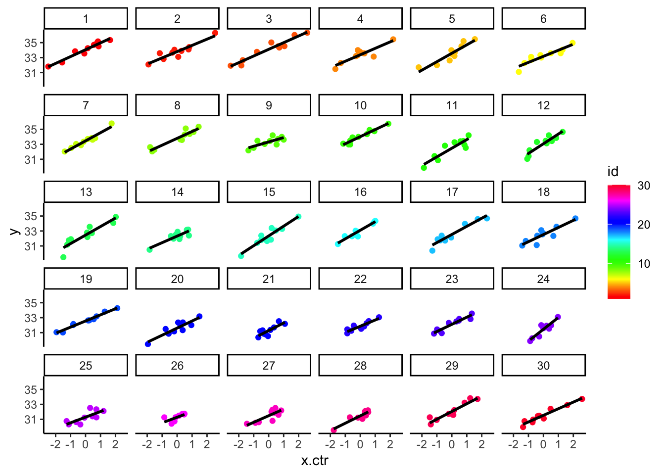 e. You can see that the upper left panel (group ID=1) starts higher and then this group level mean diminishes as we work our way towards the bottom right panel, which is group 30.
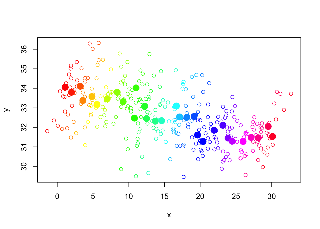
i. The shift of all of the predictors within group and the group outcome level differences are easier to see in the superimposed plot.
f. We follow this by the original data with the group means (in both x & y, superimposed), to see the contrasting emphasis.
e. You can see that the upper left panel (group ID=1) starts higher and then this group level mean diminishes as we work our way towards the bottom right panel, which is group 30.
i. The shift of all of the predictors within group and the group outcome level differences are easier to see in the superimposed plot.
f. We follow this by the original data with the group means (in both x & y, superimposed), to see the contrasting emphasis.
- While the hybrid model is an MLM, the within-group relationships can be recovered using OLS regression (NOTE: s.e. will be wrong):
##
## Call:
## lm(formula = y ~ x.ctr)
##
## Residuals:
##      Min       1Q   Median       3Q      Max
## -2.02992 -0.85285 -0.04743  0.80698  2.27159
##
## Coefficients:
##             Estimate Std. Error t value Pr(>|t|)
## (Intercept) 32.57972    0.05858  556.13   <2e-16 ***
## x.ctr        0.96619    0.06095   15.85   <2e-16 ***
## ---
## Signif. codes:  0 '***' 0.001 '**' 0.01 '*' 0.05 '.' 0.1 ' ' 1
##
## Residual standard error: 1.015 on 298 degrees of freedom
## Multiple R-squared:  0.4575, Adjusted R-squared:  0.4556
## F-statistic: 251.3 on 1 and 298 DF, p-value: < 2.2e-16- (cont.)
- The between group relationship may be recovered with OLS as we have previously shown.
6.3 Fixed vs. random effects
- The classic econometric approach: take fixed effects
- The idea is to include indicator variables for the groups – like a random effects model, only there are no distributional assumptions on the \({\eta_j}\); in fact they are estimated from the data and can be listed like any other regression parameter.
- The model is \[ {y_{ij}} = {b_0} + {b_1}{x_{ij}} + {\eta_j} + {\varepsilon_{ij}} \] \[ {\varepsilon_{ij}} \sim N(0,\sigma_\varepsilon ^2) \] If you read Gelman & Hill’s book, you might be comfortable with the idea that we could say \({\eta_j}\sim N(0,\infty)\).
- Another way to write, with indicators, is: \[ {y_{ij}} = {b_0} + {b_1}{x_{ij}} + \sum\limits_{j = 1}^J {{\eta_j}I\{ GROUP = j\} } + {\varepsilon_{ij}} \] where \(I\{\cdots\}\) is an indicator variable.
- This is no longer a classical MLM – nothing is random other than error.
- We fit this model using OLS regression:
##
## Call:
## lm(formula = y ~ factor(id) + x - 1)
##
## Residuals:
##      Min       1Q   Median       3Q      Max
## -1.52604 -0.26084 -0.00302  0.27527  0.93924
##
## Coefficients:
##              Estimate Std. Error t value Pr(>|t|)
## factor(id)1  33.00147    0.14386 229.398  < 2e-16 ***
## factor(id)2  31.87768    0.15059 211.692  < 2e-16 ***
## factor(id)3  31.00011    0.16506 187.807  < 2e-16 ***
## factor(id)4  29.91304    0.17043 175.512  < 2e-16 ***
## factor(id)5  28.88834    0.19161 150.767  < 2e-16 ***
## factor(id)6  27.80313    0.20479 135.764  < 2e-16 ***
## factor(id)7  26.70646    0.23409 114.087  < 2e-16 ***
## factor(id)8  25.69516    0.26490  96.998  < 2e-16 ***
## factor(id)9  24.41036    0.28408  85.929  < 2e-16 ***
## factor(id)10 23.37566    0.32674  71.543  < 2e-16 ***
## factor(id)11 22.04113    0.32145  68.567  < 2e-16 ***
## factor(id)12 21.26228    0.35613  59.704  < 2e-16 ***
## factor(id)13 20.37937    0.36286  56.163  < 2e-16 ***
## factor(id)14 19.07498    0.39286  48.554  < 2e-16 ***
## factor(id)15 18.23954    0.41520  43.929  < 2e-16 ***
## factor(id)16 16.98994    0.46781  36.318  < 2e-16 ***
## factor(id)17 16.00264    0.47906  33.404  < 2e-16 ***
## factor(id)18 14.99854    0.50524  29.686  < 2e-16 ***
## factor(id)19 14.05942    0.53134  26.460  < 2e-16 ***
## factor(id)20 12.64671    0.54375  23.258  < 2e-16 ***
## factor(id)21 11.56908    0.56377  20.521  < 2e-16 ***
## factor(id)22 10.65844    0.60375  17.654  < 2e-16 ***
## factor(id)23  9.71841    0.63590  15.283  < 2e-16 ***
## factor(id)24  8.36033    0.65489  12.766  < 2e-16 ***
## factor(id)25  7.65224    0.66970  11.426  < 2e-16 ***
## factor(id)26  6.16025    0.70988   8.678 3.93e-16 ***
## factor(id)27  5.27500    0.73949   7.133 9.08e-12 ***
## factor(id)28  4.29659    0.76559   5.612 4.97e-08 ***
## factor(id)29  3.53348    0.80227   4.404 1.53e-05 ***
## factor(id)30  2.42713    0.81842   2.966  0.00329 **
## x             0.96619    0.02676  36.102  < 2e-16 ***
## ---
## Signif. codes:  0 '***' 0.001 '**' 0.01 '*' 0.05 '.' 0.1 ' ' 1
##
## Residual standard error: 0.4455 on 269 degrees of freedom
## Multiple R-squared:  0.9998, Adjusted R-squared:  0.9998
## F-statistic: 5.184e+04 on 31 and 269 DF, p-value: < 2.2e-16- (cont.)
- Why does this yield the same estimates as the Hybrid model? It’s not by adjusting ‘x’ but by implicitly by adjusting ‘y’ (or the level).
- But if one adjusts y, then the relationship between x and the adjusted y changes, right? Think of adjusted y as a residualized y.
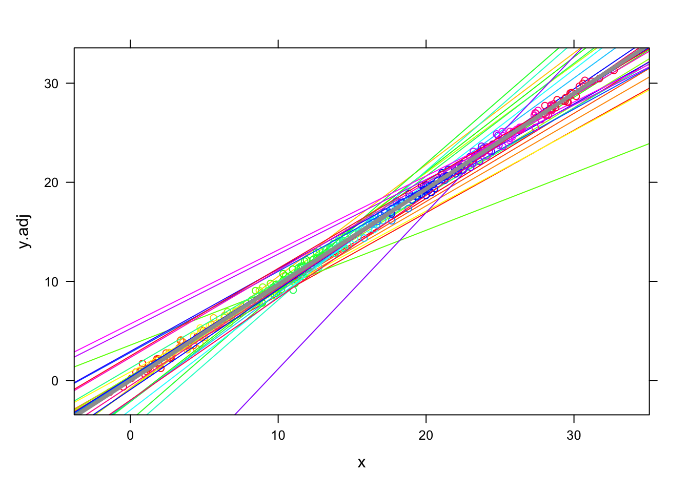
- First, recall that there are differences in level between groups, but these are not large. These adjustments are much larger because they accommodate the x effect as well. This plot is the ‘baseline’ of the information we have about relationships:
- Why does this yield the same estimates as the Hybrid model? It’s not by adjusting ‘x’ but by implicitly by adjusting ‘y’ (or the level).
Code

- (cont.)
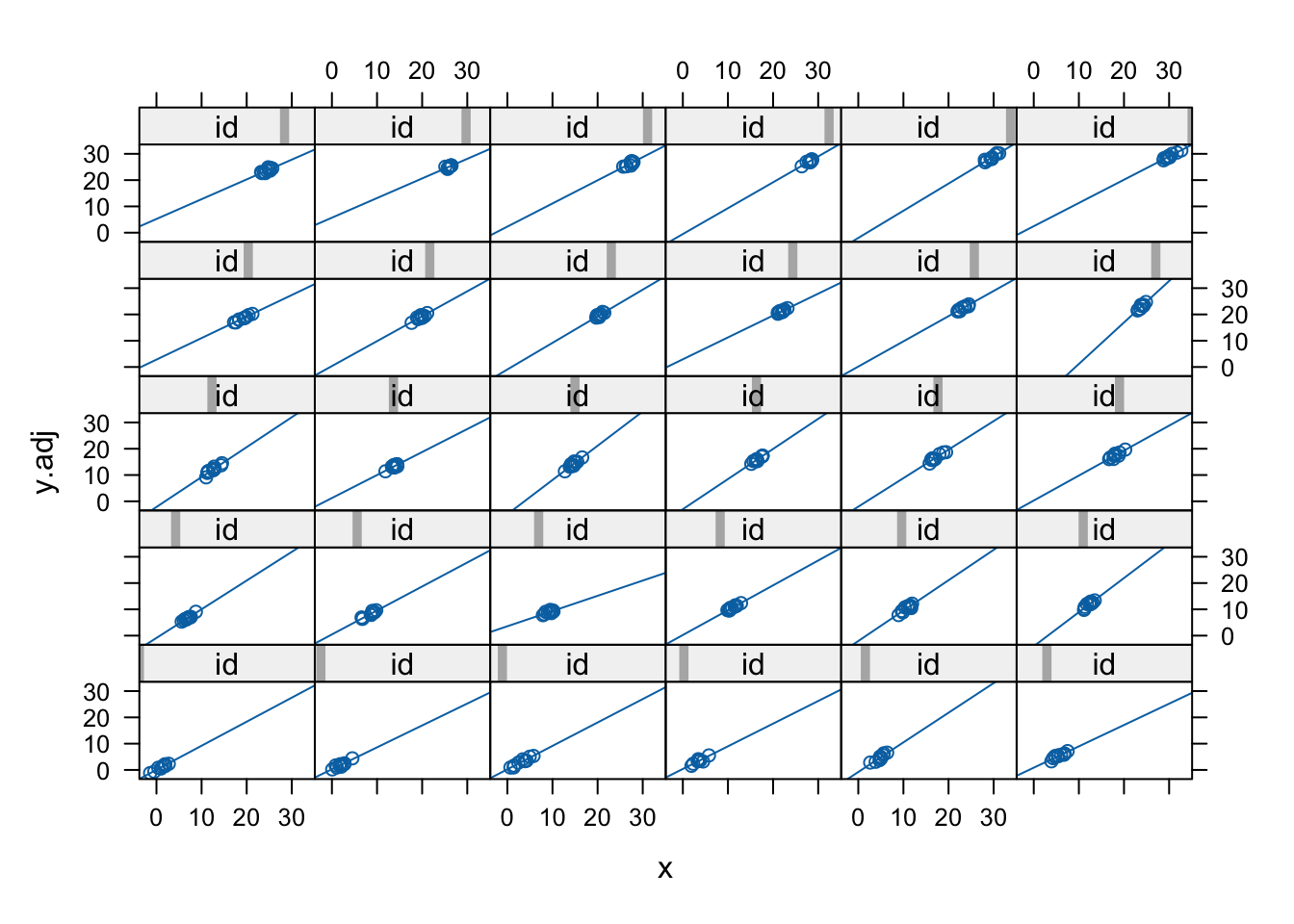
- Let’s adjust y so that the group level fixed effects \({\eta_j}\) have been removed. These are similar to residuals computed using only part of the prediction equation. So we construct \({y_{ij}} - {\eta_j}\) (ignoring x), followed by a plot of the relationships (and new level) by group:
Code
Code
## `geom_smooth()` using formula = 'y ~ x'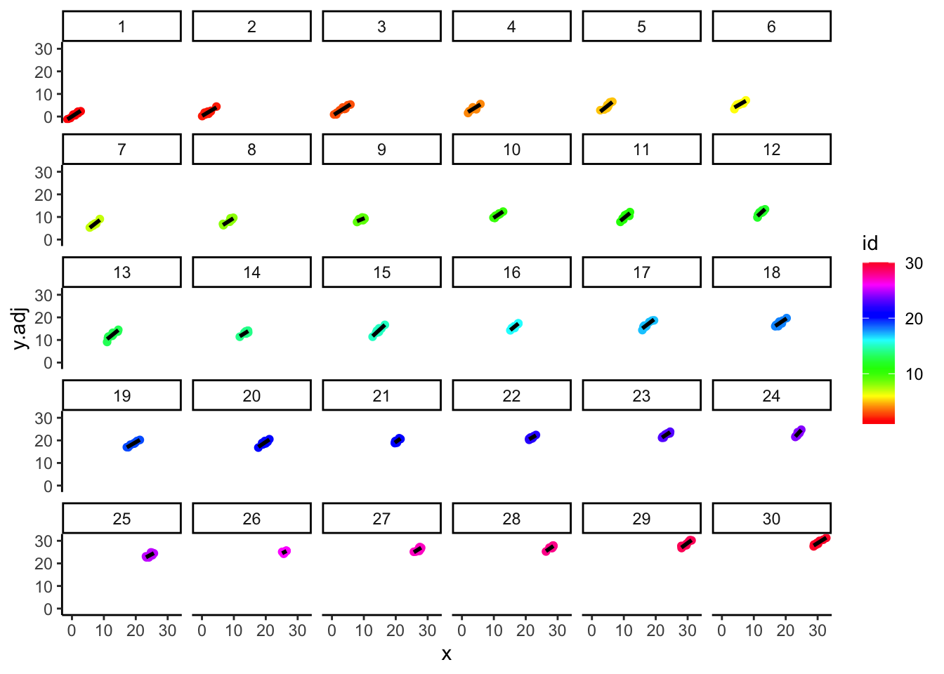
- (cont.)
- Recall that the raw differences between group outcomes is reasonably small – most are in the range 30-34.
- Above, the adjusted means are much further apart, in the range 0-30 (the fixed effect adjustments were in the range 2-33 and the constant was omitted).
- Below, we superimpose the previous plots, revealing that the adjustments align each group so that they all fall on a common regression line:
- Recall that the raw differences between group outcomes is reasonably small – most are in the range 30-34.
Code
Code
## `geom_smooth()` using formula = 'y ~ x'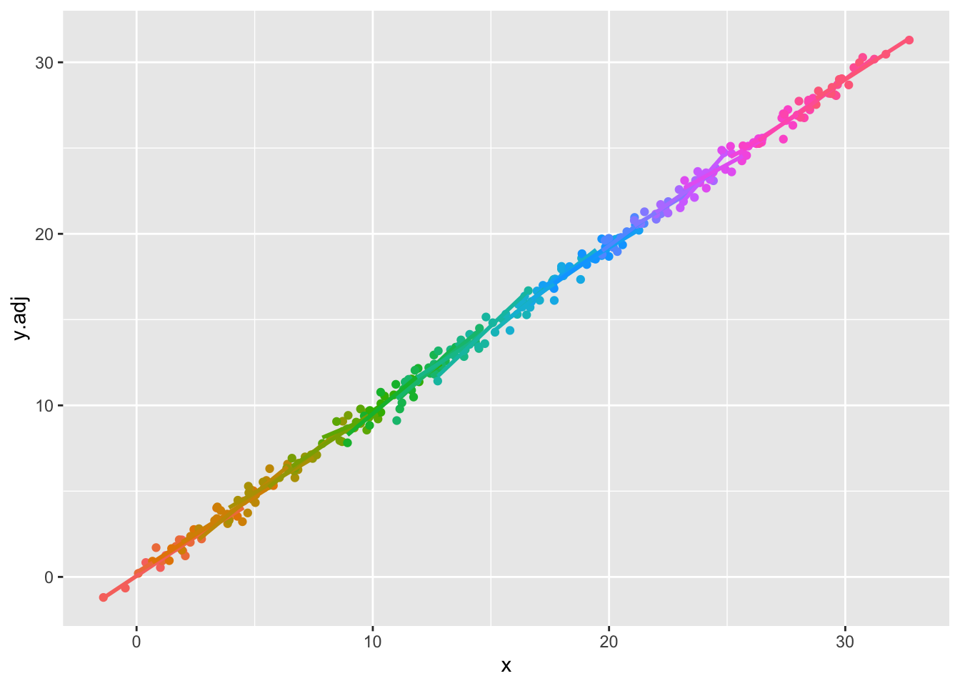
- (cont.)
- So, the fixed effects model creates an adjustment so that the outcome level moves up or down to force the adjusted values to reveal ONLY the within-group relationship (or coincide with it, depending on your perspective).
- Note that this is distinctly different than CWC, which shifts the ‘x’ to create an alignment; fixed effects models have the effect of shifting the ‘y’.
- We demonstrate this ‘motion’ in a ‘live’ animation in R:
- So, the fixed effects model creates an adjustment so that the outcome level moves up or down to force the adjusted values to reveal ONLY the within-group relationship (or coincide with it, depending on your perspective).
Code
y.it <- y
y.feff.tot <- rep(0,K) #assume FE etas are zero
liveDemo <- F
for (i in 1:300) {
  if (liveDemo) {      print(xyplot(y.it~x,group=id,type=c('p','r'),col=rainbow(K),panel=function(...) {
    panel.xyplot(...)
    panel.abline(lsfit(x,y.it),col=8,lwd=4)
  }))
    Sys.sleep(.06)
  }
  #fit model with only x
  fit.x.only <- lm(y.it~x)
  y.feff <- tapply(resid(fit.x.only),id,mean) #constr FE etas from mean resids
  y.feff.tot <- y.feff.tot + y.feff #cumulate using prior FE etas
  y.it <- y - y.feff.tot[id] #residualize by cummulative FE etas effect (recall they began as 0)
  if (i<=10 || i>290) cat(i,'beta.x=',round(coef(fit.x.only)[2],2),'sigma2.eta=',round(var(y.feff.tot),2),'\n')
}
## 1 beta.x= -0.08 sigma2.eta= 0.2
## 2 beta.x= -0.07 sigma2.eta= 0.24
## 3 beta.x= -0.06 sigma2.eta= 0.3
## 4 beta.x= -0.04 sigma2.eta= 0.38
## 5 beta.x= -0.03 sigma2.eta= 0.49
## 6 beta.x= -0.02 sigma2.eta= 0.62
## 7 beta.x= -0.01 sigma2.eta= 0.77
## 8 beta.x= 0 sigma2.eta= 0.94
## 9 beta.x= 0.02 sigma2.eta= 1.13
## 10 beta.x= 0.03 sigma2.eta= 1.34
## 291 beta.x= 0.94 sigma2.eta= 82.69
## 292 beta.x= 0.94 sigma2.eta= 82.75
## 293 beta.x= 0.94 sigma2.eta= 82.81
## 294 beta.x= 0.94 sigma2.eta= 82.86
## 295 beta.x= 0.94 sigma2.eta= 82.92
## 296 beta.x= 0.94 sigma2.eta= 82.98
## 297 beta.x= 0.94 sigma2.eta= 83.03
## 298 beta.x= 0.94 sigma2.eta= 83.09
## 299 beta.x= 0.94 sigma2.eta= 83.14
## 300 beta.x= 0.94 sigma2.eta= 83.2- (cont.)
- This iterative process keeps taking the average of the residuals from a ‘new’ set of fixed effects for each group (the etas). Each time a new adjustment is made, this yields a new relationship with ‘x’ and a new set of residuals… Eventually, only very small adjustments are made close to iteration 300…
- Why not always use fixed effects models?
- Inefficient?
- If the random effects assumptions are tenable, the fixed effects approach is unnecessary – you would get the same result and use fewer degrees of freedom.
- Many group sizes are small (or singletons)
- You care about variance components?
- You have group-constant predictors. (relates to var. comps.)
- Inefficient?
- Illustrative example: hybrid model applied to classroom data, MATHKIND outcome and SES as predictor.
- First the model with no centering: \[ MATHKIND_{ijk} = {b_0} + {b_1}SES_{ijk} + {\zeta_k} + {\varepsilon_{ijk}} \]
with the usual distributional assumptions. i. In R:
Code
## Linear mixed model fit by REML. t-tests use Satterthwaite's method ['lmerModLmerTest']
## Formula: mathkind ~ ses + (1 | schoolid)
##    Data: dat
##
## REML criterion at convergence: 12038.7
##
## Scaled residuals:
##     Min      1Q  Median      3Q     Max
## -4.7423 -0.5716  0.0188  0.6343  3.7763
##
## Random effects:
##  Groups   Name        Variance Std.Dev.
##  schoolid (Intercept)  309     17.58
##  Residual             1308     36.16
## Number of obs: 1190, groups:  schoolid, 107
##
## Fixed effects:
##             Estimate Std. Error       df t value Pr(>|t|)
## (Intercept)  465.746      2.058   98.752 226.337  < 2e-16 ***
## ses           10.722      1.589 1187.995   6.747 2.35e-11 ***
## ---
## Signif. codes:  0 '***' 0.001 '**' 0.01 '*' 0.05 '.' 0.1 ' ' 1
##
## Correlation of Fixed Effects:
##     (Intr)
## ses 0.034- (cont.)
- (cont.)
- (cont.)
- \({\hat b_1} = 10.7\); \(\hat \sigma_\zeta ^2 = 309\); \(\hat \sigma_\varepsilon ^2 = 1308\)
- (cont.)
- Preliminary data adjustment: create the school-level means for SES:
- (cont.)
Code
#*group-mean centering - setup
#egen mean_ses = mean(ses), by(schoolid)
mn.ses <- tapply(dat$ses,dat$schoolid,mean)
#gen rel_ses = ses-mean_ses
idx <- match(dat$schoolid,sort(unique(dat$schoolid)))
dat$mean_ses <- mn.ses[idx] #spreads the mean out in the right way, by idx (could use plyr library)
dat$rel_ses <- dat$ses - dat$mean_ses- (cont.)
- Now the model with group-mean centering: \[ MATHKIND_{ijk} = {b_0} + {b_{1W}}(SES_{ijk} - {\overline {SES}_k}) + {\zeta_k} + {\varepsilon_{ijk}} \] In R:
Code
## Linear mixed model fit by REML. t-tests use Satterthwaite's method ['lmerModLmerTest']
## Formula: mathkind ~ rel_ses + (1 | schoolid)
##    Data: dat
##
## REML criterion at convergence: 12049.2
##
## Scaled residuals:
##     Min      1Q  Median      3Q     Max
## -4.7714 -0.5583  0.0203  0.6253  3.7702
##
## Random effects:
##  Groups   Name        Variance Std.Dev.
##  schoolid (Intercept)  368.3   19.19
##  Residual             1304.7   36.12
## Number of obs: 1190, groups:  schoolid, 107
##
## Fixed effects:
##             Estimate Std. Error       df t value Pr(>|t|)
## (Intercept)  465.214      2.190  103.098 212.408  < 2e-16 ***
## rel_ses        9.680      1.658 1084.416   5.838 6.98e-09 ***
## ---
## Signif. codes:  0 '***' 0.001 '**' 0.01 '*' 0.05 '.' 0.1 ' ' 1
##
## Correlation of Fixed Effects:
##         (Intr)
## rel_ses 0.000- (cont.)
- (cont.)
- \({\hat b_{1W}} = 9.7\); \(\hat \sigma_\zeta ^2 = 368\); \(\hat \sigma_\varepsilon ^2 = 1305\)
- Comment: slightly smaller effect for relative (within) SES.
- Larger between-school differences.
- Relative SES doesn’t pick up as much of the school-level differences as we’d like.
- It cannot, as the overall SES level for that school has been subtracted out.
- \({\hat b_{1W}} = 9.7\); \(\hat \sigma_\zeta ^2 = 368\); \(\hat \sigma_\varepsilon ^2 = 1305\)
- Now the same model, with a group level predictor: \[ MATHKIND_{ijk} = {b_0} + {b_{1W}}(SES_{ijk} - {\overline {SES}_k}) + {b_{1B}}{\overline {SES}_k} + {\zeta_k} + {\varepsilon_{ijk}} \]
- (cont.)
Code
## Linear mixed model fit by REML. t-tests use Satterthwaite's method ['lmerModLmerTest']
## Formula: mathkind ~ rel_ses + mean_ses + (1 | schoolid)
##    Data: dat
##
## REML criterion at convergence: 12028.5
##
## Scaled residuals:
##     Min      1Q  Median      3Q     Max
## -4.8197 -0.5600  0.0096  0.6424  3.7508
##
## Random effects:
##  Groups   Name        Variance Std.Dev.
##  schoolid (Intercept)  284.9   16.88
##  Residual             1309.7   36.19
## Number of obs: 1190, groups:  schoolid, 107
##
## Fixed effects:
##             Estimate Std. Error       df t value Pr(>|t|)
## (Intercept)  466.275      2.014   93.446 231.563  < 2e-16 ***
## rel_ses        9.680      1.661 1078.518   5.827 7.46e-09 ***
## mean_ses      22.263      5.337   87.351   4.171 7.12e-05 ***
## ---
## Signif. codes:  0 '***' 0.001 '**' 0.01 '*' 0.05 '.' 0.1 ' ' 1
##
## Correlation of Fixed Effects:
##          (Intr) rel_ss
## rel_ses  0.000
## mean_ses 0.117 0.000- (cont.)
- (cont.)
- \({\hat b_{1W}} = 9.7\); \({\hat b_{1B}} = 22.3\); \(\hat\sigma_\zeta^2 = 285\); \(\hat\sigma_\varepsilon^2 = 1310\)
- Returns to relative (within) SES are the same
- The group (between), or mean SES effect is much larger.
- Test significance (of difference) using a Wald test:
- \({\hat b_{1W}} = 9.7\); \({\hat b_{1B}} = 22.3\); \(\hat\sigma_\zeta^2 = 285\); \(\hat\sigma_\varepsilon^2 = 1310\)
- (cont.)
Code
## Wald test:
## ----------
##
## Chi-squared test:
## X2 = 5.1, df = 1, P(> X2) = 0.024- (cont.)
- (cont.)
- (cont.)
- The larger group-SES effect helps to explain why the uncentered SES effect is a bit larger: in random effects MLMs without centering, the coefficient is a mixture of the relative (\({\hat b_{1W}} = 9.7\)) and group (\({\hat b_{1B}} = 22.3\)) effects.
- Note that the group means and relative SES are orthogonal, by construction, so the inclusion of one does not affect the estimate of the other.
- (cont.)
- (cont.)
- The choice between fixed and random: classical exposition (see MLM Handbook Chapter 5)
- NOTE: we are returning to a model of the form: \[ {y_{ij}} = {b_0} + {b_1}{x_{ij}}_j + {\eta_j} + {\varepsilon_{ij}} \] \[ {\varepsilon_{ij}} \sim N(0,\sigma_\varepsilon^2) \] and the assumptions surrounding \({\eta_j}\) are left to be specified.
- We are given two models: one is unbiased but inefficient; the other will be biased if its assumptions are violated, but otherwise it is more efficient. Which one should we choose?
- The fixed effects estimator is unbiased (under a limited set of assumptions, and allowing \({\eta_j}\) to vary without normality assumptions).
- The random effects estimator is efficient, and unbiased (under stronger assumptions, including that \({\eta_j}\) and \({\varepsilon_{ij}}\) are uncorrelated)
- The approach commonly used is to fit the two competing models, compare the regression coefficients, and if there is a significant, joint difference, then you have evidence that you need to use the unbiased estimator.
- Use more efficient model if no difference is detected.
- Drawbacks to using the fixed effects estimator:
- No group-constant predictors allowed
- Inefficient (even non-identifiable) – this might matter in a practical way if you don’t have enough data or replications at the group level.
- Hausman test. There are other approaches to testing fixed vs. random effects, but the Hausman test is the classical one:
- Recall that the key distinction between fixed (FE) vs. random effects (RE) models is the assumption in RE that \({\eta_j}\) and \({\varepsilon_{ij}}\) are uncorrelated (returning here to the original model ). Hausman (1978) proposes a specification test of this assumption.
- Since FE is consistent even when \({\eta_j}\) and \({\varepsilon_{ij}}\) are correlated but RE is only consistent (and more efficient) under the null of no correlation, the logic of the test is to compare the results from the two models.
- Test statistic is
- Recall that the key distinction between fixed (FE) vs. random effects (RE) models is the assumption in RE that \({\eta_j}\) and \({\varepsilon_{ij}}\) are uncorrelated (returning here to the original model ). Hausman (1978) proposes a specification test of this assumption.
\[
H = ({\hat \beta_{FE}} - {\hat \beta_{RE}})'{({\hat V_{FE}} - {\hat V_{RE}})^{ - 1}}({\hat \beta_{FE}} - {\hat \beta_{RE}})
\]
where \({\hat \beta_{FE}},{\hat \beta_{RE}}\) are the regression coefficient estimates from the FE and RE models, respectively, and \({\hat V_{FE}},{\hat V_{RE}}\) are estimates of the variance-covariance matrices associated with those coefficients.
+ This is a Wald-like test relying on the material from Handout 4 (sampling variation of parameter estimates).
3. Under the null, \(H\sim{\chi ^2}(\nu )\), where the d.f. \((\nu )\) is the number of coefficients in both models (excluding the constant).
- Worked example using the Hausman test. (NOTE: STATA and R give slightly different results) i. Fit the RE model first:
Code
- (cont.) ii. Fit the FE model next:
- (cont.)
ii. (cont.)
- Note – the FE and RE coefficients for SES are not the between groups coefficients recovered in the hybrid model. They are attempts to estimate the within-group effect.
- Both the RE & FE models are attempting to ‘control’ for group level differences.
- The difference in the coefficients for the two models is about 1 point, which is about 10% of the effect’s size.
- Here is the test statistic H:
##
##  Hausman Test
##
## data:  mathkind ~ ses
## chisq = 5.7078, df = 1, p-value = 0.01689
## alternative hypothesis: one model is inconsistent- (cont.)
iii. (cont.)
- The null is that the more efficient model (RE) is correct. This p-value suggests that there is strong evidence against this, so we should use FE models (if we only have one predictor, SES, etc.)!
- The difference didn’t look that large, but it was measured precisely enough that we reject the null, and should consider using FE models.
+ We might ‘need’ to include group-constant predictors, and this would preclude FE models, e.g.
- The null is that the more efficient model (RE) is correct. This p-value suggests that there is strong evidence against this, so we should use FE models (if we only have one predictor, SES, etc.)!
- For more details, particularly comparisons of between and within effects common to the econometric approaches to estimation, see Allison’s hybrid model discussion (2005; Fixed Effects Regression Methods for Longitudinal Data Using SAS, pp. 32-38) and Enders and Tofighi (2007), both on Brightspace.
6.4 Appendix
Useful readings
Gelman, Andrew (2005) - Why I don’t use the term “fixed and random effects”
Gelman, Andrew (2005) - ANALYSIS OF VARIANCE—WHY IT IS MORE IMPORTANT THAN EVER
6.5 Coding
lme()plm()phtest()
lme()is a function fits a linear mixed-effects model but allowing for nested random effects (allows within-group errors to be correlated / have unequal variances) fromnlmelibrary. It has arguments as follows:object: an object represents a fitted linear mixed-effects model
fixed: a two-sided linear formula object describing the fixed-effects part of the model
random: optionally, any of the following:
- a one-sided formula of the form
~ x1 + ... + xn | g1/.../gm
- a one-sided formula of the form
- a list of one-sided formulas of the form
~ x1 + ... + xn | g
- a list of one-sided formulas of the form
- a one-sided formula of the form
~ x1 + ... + xn
- a one-sided formula of the form
## Linear mixed-effects model fit by REML
##   Data: NULL
##
## Random effects:
##  Formula: ~1 | id
##         (Intercept) Residual
## StdDev:   0.3193014 1.141441
##
## Fixed effects:  y ~ x
##  Correlation:
##   (Intr)
## x -0.871
##
## Standardized Within-Group Residuals:
##         Min          Q1         Med          Q3         Max
## -2.85230865 -0.66624251 -0.02169386  0.56618706  2.47012199
##
## Number of Observations: 300
## Number of Groups: 30plm()is a function to estimate panel data of a linear model fromplmlibrary. It has arguments as follows:formula: a description for the model
index: the indexes
effect: the effects introduced in the model - one of “individual”, “time”, “twoways”, or “nested”,
model: one of “pooling”, “within”, “between”, “random” “fd”, or “ht”,
Code
phtest()is a function to test Hausman test for panel model fromplmlibrary. It has arguments as follows:x: an object of class either “panelmodel” or “formula”,
model: a character vector containing the names of two models (“within”, “random”)
effect: a character specifying the effect to be introduced to both models, one of “individual”, “time”, or “twoways”
##
##  Hausman Test
##
## data:  mathkind ~ ses
## chisq = 5.7078, df = 1, p-value = 0.01689
## alternative hypothesis: one model is inconsistent
6.6 Quiz
6.6.1 Self-Assessment
Use “W6 Activity Form” to submit your answers.
- Given the Data Generating Process (DGP) described in Chapter 6 1.b.iii:
1-A: Are any of the assumptions of MLMs violated by the DGP?
1-B: Is the correlation between \(X_{ij}\) and \(\eta_{j}\) positive or negative? Is it an MLM assumption for them to be independent?
1-C: If you were to run separate regressions for each group (indicated by the colors in the plot), what would the relationship be (negative or positive)?
1-D: What would the relationship be if you ignore the colors? Is this completely pooled or an unpooled approach?
- Given the model as follows:
\[ y_{ij} = b_0 + b_1(x_{ij} - \bar x_j) + b_2\bar x_j + \eta_j + \epsilon_{ij} \]
2-A: Describe all of the terms in the equation.
2-B: Is this still an MLM? Why or why not?
2-C: Why isn’t it “redundant” or collinear to have both \(x_{ij} - \bar x_j\) and \(\bar x_j\) in the same model?
- Given the Data Generating Process (DGP) described in chapter 6 1.b.iii and the fixed effects model given by this R code:
fit.fe <- lm(y~factor(id)+x-1)different from an MLM? Be sure to discuss as follows:
3-A: What are the predictors in the model?
3-B: What are parameters including their number?
3-C: What are assumptions?
6.6.2 Lab Quiz
- Review the material in the Rshiny app “Week6: Handout6 Activity” and then answer these questions on the google form “W6 Activity Form”
6.6.3 Homework
- Homework is presented as the last section of the Rshiny app “Week6: Handout6 Activity”.
- Follow instructions there (fill out this form “W6 Activity Form” ) and hand in your code on Brightspace