Chapter 2 : MLM conceptualization
Code
2.1 MLM conceptualization, notation and effects
2.1.1 Classroom data example
- Even though three levels of nesting are present in our classroom data, we now conceptualize MLMs using a simpler model containing an individual-level predictor and effects only for schools (we will eventually bring classrooms back into the picture):
- This is the model under consideration: \(Y_{ijk} = b_0 + b_1 X_{1ijk} + \zeta_k + \varepsilon_{ijk}\); \(\zeta_k\sim N(0,\sigma^2_\zeta)\) independent of \(\varepsilon_{ijk}\sim N(0,\sigma^2_\epsilon)\).
- We now work through some different conceptualizations of the components of this model structure. Each one contributes different insight into what it means to include random effects in a model.
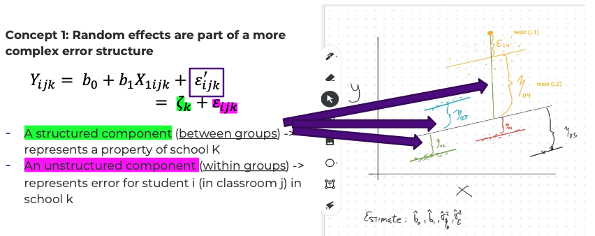
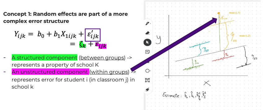
- Conceptualization #1: random effects are part of a more complex error structure.
- Let \(\varepsilon_{ijk}' = \zeta_k + \varepsilon_{ijk}\) . Then \(Y_{ijk} = b_0 + b_1 X_{1ijk} + \varepsilon_{ijk}'\) – the second equation sure looks a lot like ‘plain old’ regression. But these new error terms are not independent across subjects in the same school.
- The error term \(\varepsilon_{ijk}'\) has two parts:
- A structured component \(\zeta_k\) (between groups)
- An unstructured component \(\varepsilon_{ijk}\) (within groups)
- The indices (subscripts) tell us a lot about what type of variation we are identifying:
- \(\zeta_k\) represents a property of school k (‘error’ for the school?)
- \(\varepsilon_{ijk}\) represents error for student i (in classroom j) in school k
- Returning to the term \(\zeta_k + \varepsilon_{ijk}\), the fact that \(\zeta_k\) ‘repeats’ across observations in the same school captures a form of dependence with certain properties:2
- Covariance between errors from students in the same school: \[ Cov(\varepsilon_{ijk}',\varepsilon_{i'j'k}') = Cov(\zeta_k + \varepsilon_{ijk},\zeta_k + \varepsilon_{i'j'k}) \] \[ = Cov(\zeta_k,\zeta_k)+Cov(\varepsilon_{ijk},\varepsilon_{i'j'k})+Cov(\zeta_k,\varepsilon_{ijk})+Cov(\zeta_k,\varepsilon_{i'j'k}) \] \[ = Var(\zeta_k)+0+0+0 = \sigma^2_\zeta \mbox{ (not zero!)} %\mbox{ by all of our assumptions} \]
- Note as well that \(Var(\varepsilon_{ijk}') = Var(\zeta_k)+Var(\varepsilon_{ijk})+2Cov(\zeta_k,\varepsilon_{ijk})=\sigma^2_\zeta+\sigma^2_\varepsilon = Var(\varepsilon_{i'j'k}')\).
- The cross-product (covariance) terms in the variance calculation are zero, so it is just the sum of two variances.
- This implies that \(Cor(\varepsilon_{ijk}',\varepsilon_{i'j'k}') = \frac{\sigma^2_\zeta}{(\sqrt{\sigma^2_\zeta+\sigma^2_\varepsilon})^2}\), which corresponds to our measure of the proportion of variation that is between schools (ignoring classrooms). It is also the formula for the Intraclass Correlation Coefficient (ICC). Reminder: make note of this formula (you have seen it in Handout 1 as well). 1. We have just shown that – net of the mean, so holding the predictors constant – the ICC is the correlation between a random pair of observations within the same school (k), induced by our model.
- Identification: we can learn about \(\zeta_k\) for a specific school k, and identify the effect, by looking for systematic, mean differences in level for all students in that school. HERE IS A WAY TO CONCEPTUALIZE THIS: Imagine that you ran OLS regression on your outcome, ignoring the nested nature of your data. If, for some schools, the structured error terms \(\{\varepsilon_{ijk}'\}_{\cdot k}\) (there are many of these; this is a notation for all errors (including the structured part) for school k, as we have defined them) are typically ‘high,’ while for other schools they are typically low, then we can associate those high or low levels with each school through component \(\zeta_k\).
- We will do this, constructively, in a section that follows.
- We will do this, constructively, in a section that follows.
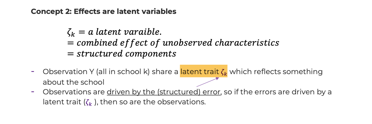
- Conceptualization #2: effects are latent variables
- Some insight can be gained if one thinks of \(\zeta_k\) as a latent variable, which is a fancy way of saying the combined effect of unobserved characteristics.
- We sometimes say that observations \(Y_{ijk}\), all in school k, share a latent trait \(\zeta_k\) that reflects something about the school.
- Observations are driven by the (structured) error, so if the errors are driven by a latent trait, then so are the observations.
- This can be characterized (for the structured errors) by a path diagram (for the same school k):
- The latent trait \(\zeta_k\) is shared by structured error terms, \(\varepsilon_{ijk}',\varepsilon_{i'j'k}'\), and thus outcomes, \(Y_{ijk},Y_{i'j'k}\).
- Some insight can be gained if one thinks of \(\zeta_k\) as a latent variable, which is a fancy way of saying the combined effect of unobserved characteristics.
- Conceptualization #3: random coefficients
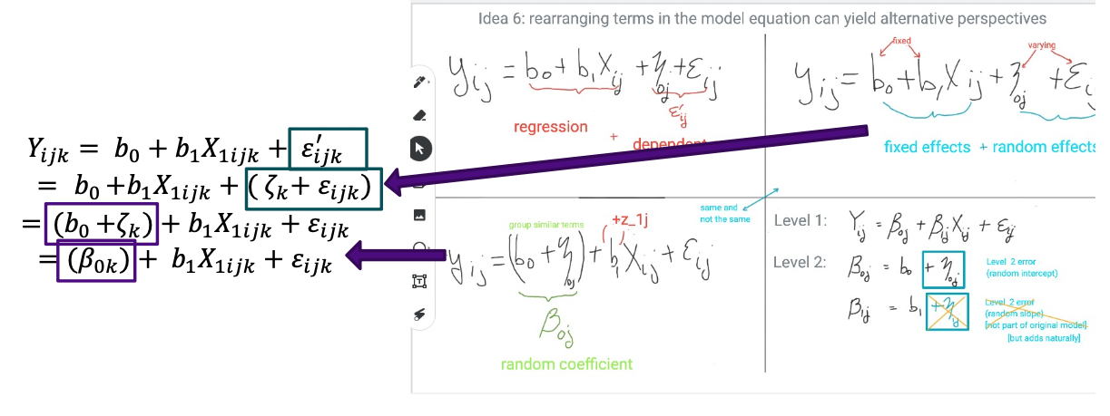
- We can regroup the terms in the complex error:
- Starting with \({Y_{ijk}} = {b_0} + {b_1}{X_{1ijk}} + {\varepsilon '_{ijk}}\), we substitute in the expression for the error: \({Y_{ijk}} = {b_0} + {b_1}{X_{1ijk}} + ({\zeta_k} + {\varepsilon_{ijk}})\)
- And now regroup: \({Y_{ijk}} = ({b_0} + {\zeta_k}) + {b_1}{X_{1ijk}} + {\varepsilon_{ijk}}\).
- And finally, rename & re-index: \({Y_{ijk}} = ({\beta_{0k}}) + {b_1}{X_{1ijk}} + {\varepsilon_{ijk}}\), where \({\beta_{0k}} = {b_0} + {\zeta_k}\).
- The term \({\beta_{0k}} = {b_0} + {\zeta_k}\) is a ‘random coefficient’ (or random intercept) that varies by school, not by student i in school, or even by classroom (yet).
- Every student in school k has regression intercept \({\beta_{0k}}\), not just plain old \({b_{0}}\). Since k can vary across all possible school indices, this yields many school-specific intercepts.
- This is not the same as running separate regressions for each school. (crucial to understand why)
- There are different ways to describe this formulation: random coefficients, random regression. It is also closely aligned with ‘hierarchical’ or ‘level’ notation, to be introduced next.
- We can regroup the terms in the complex error:
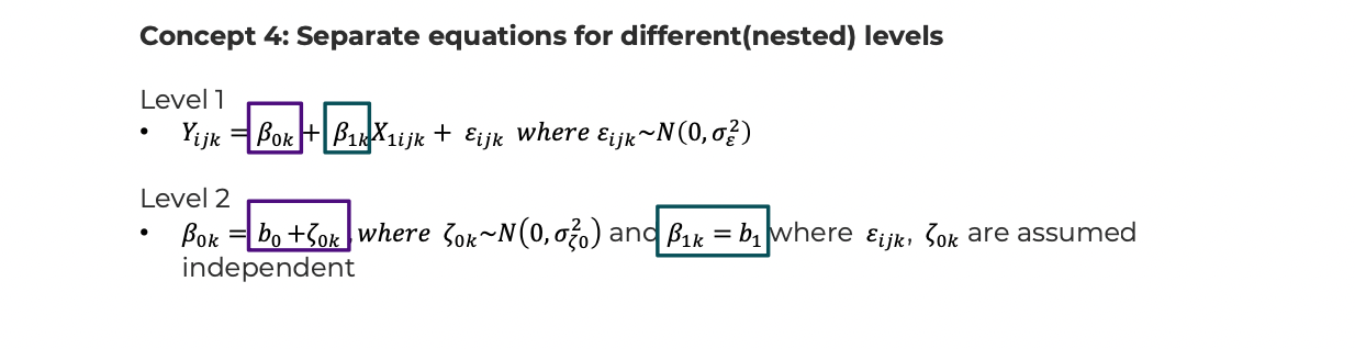
- Conceptualization #4, separate equations for different (nested) levels.
- School data is naturally hierarchical, and we have already introduced predictors that vary at different “levels” of the nested data structure. We now make this explicit through the use of notation.
- First, we copy the re-indexed version of our model presented in Section 4, and call this “level 1”:
- Level 1 is the topmost level and terms that are listed should require the maximal number of subscripts. With nested data, it is usually the subject level, as in outcome \({Y_{ijk}}\).
- Level 1: \({Y_{ijk}} = {\beta_{0k}} + {\beta_{1k}}{X_{1ijk}} + {\varepsilon_{ijk}}\), \({\varepsilon_{ijk}} \sim N(0,\sigma_\varepsilon ^2)\)
- There are many terms in this equation that vary by school: the outcome, the predictor, the error, the intercept and the slope on the predictor. That’s right, the intercept and slope are school-specific. If we assign a distribution to the intercept term (only) such that it is based on a random variable, such as a draw from a normal distribution, we call this a random intercepts model.
- We further specify terms such as \({\beta_{0k}}\) at ‘lower’ levels, in this case level 2 will be used.
- Level 2: \({\beta_{0k}} = {b_0} + {\zeta_{0k}}\), \({\zeta_{0k}} \sim N(0,\sigma_{{\zeta_0}}^2)\), and \({\beta_{1k}} = {b_1}\), where \({\varepsilon_{ijk}},{\zeta_{0k}}\) are assumed independent. The ‘0’ in the subscript allows for naming additional random effects; e.g., \(\zeta_{1k}\) or \(\zeta_{2k}\).
- Each of these equations can be made more or less complex. For example, we can remove the level 2 error term, \({\zeta_{0k}}\) (yes, this is an error term, but a structured or group-level error term), and then we have regression, ignoring any correlation structure in the errors:
- Level 1: \({Y_{ijk}} = {\beta_{0k}} + \beta_{1k} X_{1ijk} + {\varepsilon_{ijk}}\), \({\varepsilon_{ijk}} \sim N(0,\sigma_\varepsilon ^2)\)
- Level 2: \({\beta_{0k}} = {b_0}\); \({\beta_{1k}} = {b_1}\)
- Why go to so much trouble, notationally?
- The levels are organized directly around the nesting principle (an example follows soon).
- There are “rules” associated with what can be included (predictors and error terms) at each level, ensuring some quality control (fewer coding/conceptualizing mistakes).
- There is a sense that each equation is a mini-regression, and as such, one can think about explaining variation at different levels with different equations.
- The notation is extremely common in much of the literature.
- Two software packages, HLM and MLwiN are based on this organizing principle.
- Moving between this notation and the alternative, used by STATA/SAS/R simply involves algebraic substitution.
2.1.2 A constructive approach to random effects, or, what are these things we call ‘effects’?
- Returning to the structured errors perspective, how can we construct \(\zeta_k\) “by hand”?
- Recall conceptualization #1: according to that model, the errors from a regression look like this: \(\varepsilon_{ijk}' = \zeta_k + \varepsilon_{ijk}\). We can’t easily separate the two components (yet), but we can look at their sum.
- The same way one examines residuals to evaluate potential omitted variables, one can use them to evaluate potential omitted “structured error” (the term \(\zeta_k\)).
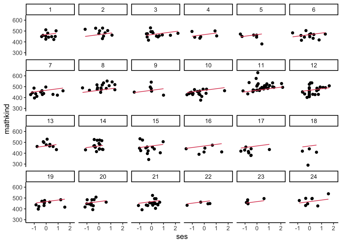
- Below, we run a simple OLS regression of MATHKIND on SES, generate the regression line (using a predict command), and then plot the raw observations against the common, or pooled, regression line for the first 24 schools to show that some seem to have residuals typically above or below the regression line.
- Recall conceptualization #1: according to that model, the errors from a regression look like this: \(\varepsilon_{ijk}' = \zeta_k + \varepsilon_{ijk}\). We can’t easily separate the two components (yet), but we can look at their sum.
##
## Call:
## lm(formula = mathkind ~ ses, data = dat)
##
## Residuals:
##      Min       1Q   Median       3Q      Max
## -174.835  -26.399    1.065   26.529  161.150
##
## Coefficients:
##             Estimate Std. Error t value Pr(>|t|)
## (Intercept)  466.845      1.162  401.70   <2e-16 ***
## ses           14.359      1.568    9.16   <2e-16 ***
## ---
## Signif. codes:  0 '***' 0.001 '**' 0.01 '*' 0.05 '.' 0.1 ' ' 1
##
## Residual standard error: 40.08 on 1188 degrees of freedom
## Multiple R-squared:  0.06596,    Adjusted R-squared:  0.06518
## F-statistic:  83.9 on 1 and 1188 DF,  p-value: < 2.2e-16
Code
- It is a bit hard to ‘see’ what the average shift up or down would be at the school level. Maybe a boxplot will reveal some of the structure (this time, we generate residuals directly):
Code
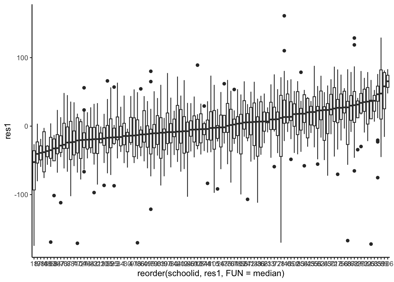
- (cont.) i. We do see a fair amount of variation in the level, represented by the median residual for each school. ii. If the errors were dependent errors, we’d see structure (and we do). This observation is crucial: if the errors were independent, the medians would be much closer to zero for every school.3
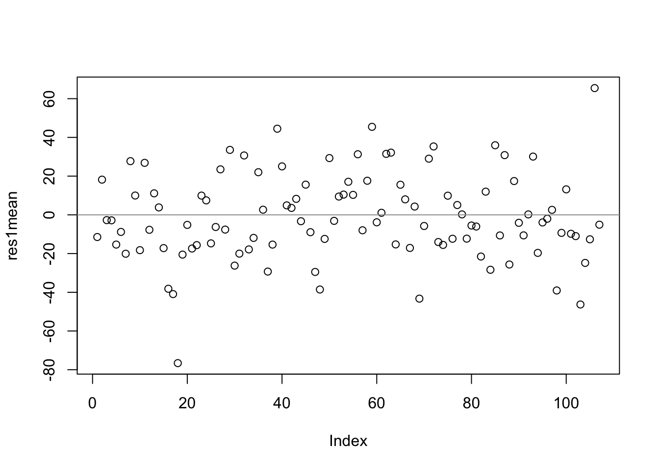
- Let’s take the average of these residuals at the school level and use them as a first approximation—an estimate of \(\zeta_k\).
- This code generates a school-level mean residual:
We visualize these average residuals by case number in the reduced file (this x-axis is meaningless, but useful to spread the observations apart).
- (cont.)
- (cont.)
- The main point of this plot is that different schools have different mean residuals. This is not ‘evidence’ of homoscedasticity (though the picture looks similar), as (1) there is only one data point per school, so they do not represent variance; (2) the data points are averages of residuals; (3) the x-axis is arbitrary.
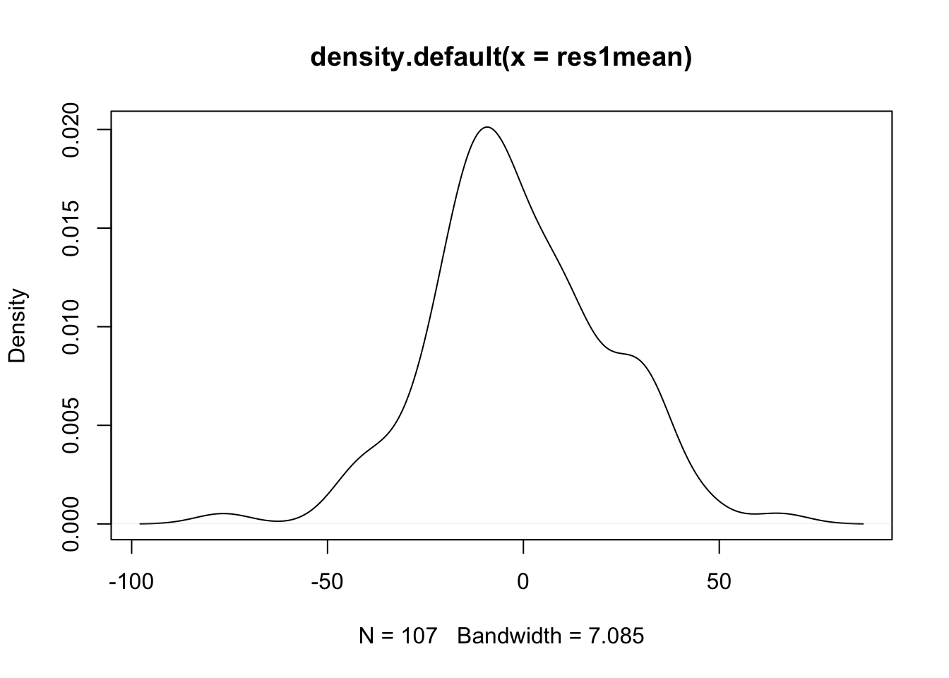
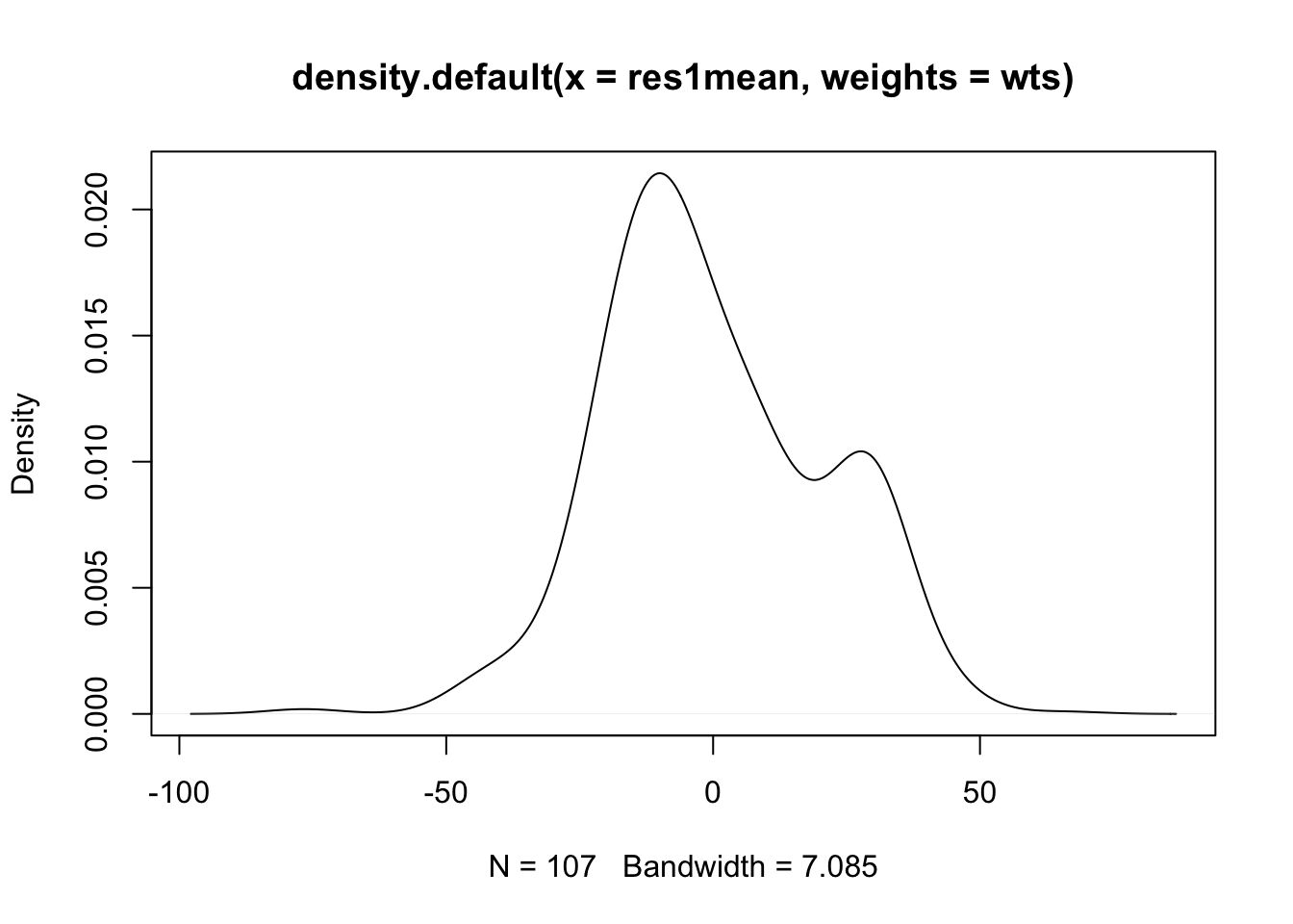
- These estimates of have a distribution (as they vary by school), which we can examine with density plots and by calculating the standard deviation (square root of variance).
- (cont.)
- (cont.)
- The standard deviation is pretty large at 22.43
- If you used STATA, and egen, you would see a bimodialty in this plot, as the mean is assigned to every student in that school. If we wish to weight by the number of students sampled in each school, we could do it in several ways in R, but let’s try using the weights option of the density function.
Code
- (cont.)
- And there is the bimodality you would get in STATA (there are ways to correct it of course).
- While the ‘default’ R method
tapplydid what we wanted, it is instructive to see how this might have looked if one were less aware of these software differences. Of course, one could wish to weight by school size as well.
- Summarizing, we constructed ‘crude’ estimates of the structured, school-level error component \({\zeta_k}\) using average residuals.
- The distribution was reasonably symmetric (when the distribution was computed with one observation per school). We computed the std. dev. of these terms, which was about 20 or 22. This is a crude estimate of the variance component \(\sigma_\zeta ^2\).
- We now run a mixed model to see a better estimate of variance component (shortly, we’ll see why it’s ‘better’)
## Linear mixed model fit by REML. t-tests use Satterthwaite's method ['lmerModLmerTest']
## Formula: mathkind ~ ses + (1 | schoolid)
##    Data: dat
##
## REML criterion at convergence: 12038.7
##
## Scaled residuals:
##     Min      1Q  Median      3Q     Max
## -4.7423 -0.5716  0.0188  0.6343  3.7763
##
## Random effects:
##  Groups   Name        Variance Std.Dev.
##  schoolid (Intercept)  309     17.58
##  Residual             1308     36.16
## Number of obs: 1190, groups:  schoolid, 107
##
## Fixed effects:
##             Estimate Std. Error       df t value Pr(>|t|)
## (Intercept)  465.746      2.058   98.752 226.337  < 2e-16 ***
## ses           10.722      1.589 1187.995   6.747 2.35e-11 ***
## ---
## Signif. codes:  0 '***' 0.001 '**' 0.01 '*' 0.05 '.' 0.1 ' ' 1
##
## Correlation of Fixed Effects:
##     (Intr)
## ses 0.034- (cont.)
- The variance component estimate (as s.d.) is \(\hat{\sigma}_\zeta=\) which is a bit smaller than our prior estimates.
- Adding in a second level of nesting
- Returning to the more complex setup: \(Y_{ijk} = b_0 + b_1 X_{1ijk} + \eta_{jk} + \zeta_k + \varepsilon_{ijk}\), we again rewrite the error term, now with three components: \(\varepsilon'_{ijk} = \eta_{jk} + \zeta_k + \varepsilon_{ijk}\), and simpler model form: \(Y_{ijk} = b_0 + b_1 X_{1ijk} + \varepsilon '_{ijk}\)
- The average \(\varepsilon'_{ijk}\) aggregated by schools still gives us a rough estimate of \({\zeta_k}\).
- What if we start with this equation, \(\varepsilon'_{ijk} = \eta_{jk} + \zeta_k + \varepsilon_{ijk}\), and subtract \(\zeta_k\) from both sides? Then we have: \(\varepsilon'_{ijk}-\zeta_k = \eta_{jk} + \varepsilon_{ijk}\). In other words, we are left with classroom and student level errors, only.
- Averaging estimates of this differenced form of the error, \(\eta_{jk} + \varepsilon_{ijk}\), by classroom could yield rough estimates of \(\eta_{jk}\), because we assume that the mean for \(\varepsilon_{ijk}\) is zero, at the classroom or any level of aggregation.
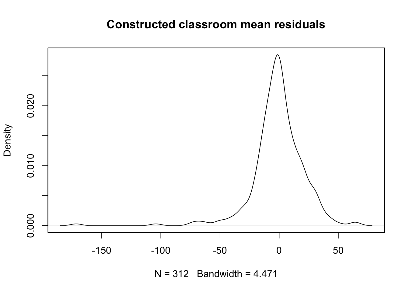
- We want to construct classroom level ‘effects,’ using available residuals.
- The first step is to subtract estimates of the school-level mean residual from the overall residual, following this equation: \(\varepsilon'_{ijk}-\zeta_k=\eta_{jk} + \varepsilon_{ijk}\)
- We then take the means of estimates of \(\varepsilon'_{ijk}-\zeta_k\), by classroom, much as we did to create means by schoolid. But the means are of a residual that has already been cleared of ‘school effects’.
- We briefly explore this here.
Code
- Comments
- The estimated standard deviation within classrooms, net of mean-school-residual effects is 22.12. Very large.
- In a classroom with only one student, separating the structured error is problematic – actually all of the ‘effect’ will be allocated to the structured error, leading to larger estimates of its variance.
- The above approach (taking mean residuals by groups) is roughly equivalent to the econometric approach known as “fixed effects”. It clearly overestimates the effects for groups with one observation, but the imprecision of the estimates may also be a concern for small group sizes.
- Running a mixed effects model is the proper approach in many nested data applications. We now run a mixed model for three levels of nesting.
## Linear mixed model fit by REML. t-tests use Satterthwaite's method ['lmerModLmerTest']
## Formula: mathkind ~ ses + (1 | schoolid/classid)
##    Data: dat
##
## REML criterion at convergence: 12038.4
##
## Scaled residuals:
##     Min      1Q  Median      3Q     Max
## -4.7444 -0.5722  0.0112  0.6320  3.7507
##
## Random effects:
##  Groups           Name        Variance Std.Dev.
##  classid:schoolid (Intercept)   20.44   4.521
##  schoolid         (Intercept)  301.52  17.364
##  Residual                     1294.08  35.973
## Number of obs: 1190, groups:  classid:schoolid, 312; schoolid, 107
##
## Fixed effects:
##             Estimate Std. Error       df t value Pr(>|t|)
## (Intercept)  465.749      2.058   99.030 226.344  < 2e-16 ***
## ses           10.684      1.589 1187.053   6.725 2.72e-11 ***
## ---
## Signif. codes:  0 '***' 0.001 '**' 0.01 '*' 0.05 '.' 0.1 ' ' 1
##
## Correlation of Fixed Effects:
##     (Intr)
## ses 0.035- (cont.)
- Even in a doubly nested model, our previously constructed, residual-based mean school effects seem to overestimate the variance components.
- Residual-based estimates are particularly susceptible to what is sometimes called, “following the noise,” which is clear when there is only one student in a classroom – there is simply no way to isolate the structured from unstructured error, so this rough approach puts all of the error into the structured component.
- Even in a doubly nested model, our previously constructed, residual-based mean school effects seem to overestimate the variance components.
2.1.3 Model Selection
- Comparing nested models
- A common way to determine what components of a model are necessary (fixed effects or random effects), from a statistical perspective, is to conduct a significance test on some subset of the model’s parameters. The test we have already introduced and will use extensively is a likelihood ratio test (LRT or LR test).
- In this setting, parameters are added to an existing model, establishing a “nesting” of one model in the other that facilitates the LR test.
- When all of the parameters considered are regression coefficients (fixed effects), then the tests are for statistical differences from zero, either singly, or as a vector. T-tests of single coefficents and Wald tests for blocks of coefficients may be used.
- A common way to determine what components of a model are necessary (fixed effects or random effects), from a statistical perspective, is to conduct a significance test on some subset of the model’s parameters. The test we have already introduced and will use extensively is a likelihood ratio test (LRT or LR test).
- Selecting random effects (first pass)
- A natural consideration in building mixed effects models is the presence and complexity of the random effects.
- The very first question to ask is whether any random effects are needed. We will use the classroom data, beginning with a model for MATHGAIN with no covariates: \(MATHGAIN_{ijk} = {b_0} + \zeta_k+ \varepsilon_{ijk}\), with \({\zeta_k} \sim N(0,\sigma_\zeta ^2)\) and \({\varepsilon_{ijk}} \sim N(0,\sigma_\varepsilon ^2)\) independently of one another. Recall that this is called the unconditional means model. The ‘extra’ subscripts are intentionally included, as they will become important as we add random effects for classrooms.
- We want to use an LRT to compare a model with no random effects to one with random effects for schools, but it can be challenging to fit a model with no random effects (yes, this is plain old regression, but we need to be able to compare likelihoods, and that isn’t set up (in a simple manner) under R’s lm and lmer functions, so we instead have to use the function
ranovain the lmerTest library in R).
- We want to use an LRT to compare a model with no random effects to one with random effects for schools, but it can be challenging to fit a model with no random effects (yes, this is plain old regression, but we need to be able to compare likelihoods, and that isn’t set up (in a simple manner) under R’s lm and lmer functions, so we instead have to use the function
## ANOVA-like table for random-effects: Single term deletions
##
## Model:
## mathgain ~ (1 | schoolid)
##                npar  logLik   AIC    LRT Df Pr(>Chisq)
## <none>            3 -5888.3 11783
## (1 | schoolid)    2 -5904.8 11814 32.881  1  9.796e-09 ***
## ---
## Signif. codes: 0 '***' 0.001 '**' 0.01 '*' 0.05 '.' 0.1 ' ' 1- A more interesting comparison would be whether we need to add a random classroom effect, after controlling for school effects, and this is an LRT.
- If we add random classroom effects to the last model and then compare likelihoods with an LRT, we have an answer to this question.
- The model to examine is \(MATHGAIN_{ijk} = {b_0} + \eta_{jk} + \zeta_k+ \varepsilon_{ijk}\), with the usual normality and independence assumptions on all random terms.
## Data: dat
## Models:
## lmer.fit2: mathgain ~ (1 | schoolid)
## lmer.fit3: mathgain ~ (1 | schoolid/classid)
##           npar   AIC   BIC  logLik deviance  Chisq Df Pr(>Chisq)
## lmer.fit2    3 11783 11798 -5888.3    11777
## lmer.fit3    4 11777 11797 -5884.4    11769 7.9048  1    0.00493 **
## ---
## Signif. codes: 0 '***' 0.001 '**' 0.01 '*' 0.05 '.' 0.1 ' ' 1- (cont.)
- (cont.)
- (cont.)
- We used the
anovacommand, which does a sequential LRT based on the listed model fits. - The chi-square test, on one degree of freedom (corresponding to the additional variance component) is highly significant, with p<0.01. Conclusion: inclusion of classroom effects is warranted.
- Question: can we use the LRT given by ranova() applied to the more complex model? Answer: That function divises two LR tests; it is likely that we can find the test that we require (see R code that follows).
- Question: I thought we found, previously, that the classroom effects were not needed? Why does this result differ?
- We used the
- (cont.)
- (cont.)
## ANOVA-like table for random-effects: Single term deletions
##
## Model:
## mathgain ~ (1 | classid:schoolid) + (1 | schoolid)
##                        npar  logLik   AIC    LRT Df Pr(>Chisq)
## <none>                    4 -5884.4 11777
## (1 | classid:schoolid)    3 -5888.3 11783 7.9048  1   0.004930 **
## (1 | schoolid)            3 -5888.3 11783 7.8875  1   0.004978 **
## ---
## Signif. codes: 0 '***' 0.001 '**' 0.01 '*' 0.05 '.' 0.1 ' ' 1- LRTs for mixed effects models: comparing fixed effects parameters.
- Many mixed effects models are fit using ‘restricted’ maximum likelihood (REML). This is the default in R; no longer default in STATA v.14+
- Researchers prefer REML over what is sometimes referred to as “full” ML or FML because the estimation of variance components is unbiased using REML.
- Unfortunately, we cannot use LR tests to compare the fixed effects of models fit under REML (there is another way, to be given soon).
- If you try to use REML fits to compare fixed effects, R will refit the model using FML; STATA will ‘warn’ you with an error.
- When the comparison of interest involves the fixed effects, you can force the fit to use FML, by choosing MLE as an option to the call to STATA’s xtmixed (or in R you can let the functions that compare models call the ‘refitting’ procedure).
- We normally do not compare models that change both fixed and random effects at the same time, but it is possible under FML.
- Note: if you are evaluating the inclusion of a single, continuous predictor to a model, you can just look at the p-value (fixed effects output).
- Here, we explore the assessment of ‘blocks’ of predictors.
- Example: let’s add SES and (teacher-level) MATHKNOW to our model as a ‘block’ and evaluate whether either is significant (the null hypothesis is that the regression coefficients for both are identically zero).
- The new model is: \(MATHGAIN_{ijk} = {b_0} + b_1 SES_{ijk} + b_2 MATHKNOW_{jk} + \eta_{jk} + \zeta_k + \varepsilon_{ijk}\), with the usual normality and independence assumptions on all random terms, and will be compared to the model fit in the prior section.
- We first do this naively, using REML:
- Many mixed effects models are fit using ‘restricted’ maximum likelihood (REML). This is the default in R; no longer default in STATA v.14+
## Linear mixed model fit by REML. t-tests use Satterthwaite's method ['lmerModLmerTest']
## Formula: mathgain ~ ses + mathknow + (1 | schoolid/classid)
##    Data: dat
##
## REML criterion at convergence: 10684.6
##
## Scaled residuals:
##     Min      1Q  Median      3Q     Max
## -4.3702 -0.6106 -0.0342  0.5357  5.5805
##
## Random effects:
##  Groups           Name        Variance Std.Dev.
##  classid:schoolid (Intercept)  104.64  10.229
##  schoolid         (Intercept)   92.11   9.598
##  Residual                     1018.67  31.917
## Number of obs: 1081, groups:  classid:schoolid, 285; schoolid, 105
##
## Fixed effects:
##              Estimate Std. Error        df t value Pr(>|t|)
## (Intercept)   57.8169     1.5468   91.6576  37.379   <2e-16 ***
## ses            0.8847     1.4602 1039.2449   0.606   0.5447
## mathknow       2.4341     1.3093  211.2083   1.859   0.0644 .
## ---
## Signif. codes:  0 '***' 0.001 '**' 0.01 '*' 0.05 '.' 0.1 ' ' 1
##
## Correlation of Fixed Effects:
##          (Intr) ses
## ses       0.039
## mathknow 0.009 -0.042## Error in anova.merMod(lmer.fit3, lmer.fit4, refit = F) :
## models were not all fitted to the same size of dataset
## [1] "Error in anova.merMod(lmer.fit3, lmer.fit4, refit = F) : \n models were not all fitted to the same size of dataset\n"
## attr(,"class")
## [1] "try-error"
## attr(,"condition")
## <simpleError in anova.merMod(lmer.fit3, lmer.fit4, refit = F): models were not all fitted to the same size of dataset>- (cont.)
- It doesn’t quite look like SES or MATHKNOW is significant, but we don’t really know if they are jointly non-significant until we do the proper test in the
anova, but … - The test we thought we could do ‘fails’ for a different reason: the problem occurred because in fitting a model with more predictors, we lost nine cases due to missingness. LRTs are only legitimate when the included observations are the same in both models.
- To remedy the situation, we can choose a subsample of observations from the dataset before performing the model estimation. We can identify which observations were included in the model by establishing an indicator variable (‘in_sample’) with that information:
- It doesn’t quite look like SES or MATHKNOW is significant, but we don’t really know if they are jointly non-significant until we do the proper test in the
Code
save.options <- options() #so that old options can be restored
options(na.action='na.pass')
mm <- model.matrix(~mathgain+ses+mathknow,data=dat)
in_sample <- apply(is.na(mm),1,sum)==0 # these rows aren't missing anything
options(save.options)
#re-fit mlms using only fully observed observations, even in model with fewer predictors.
fit7 <- lmer(mathgain~1+(1|schoolid/classid),data=dat,subset=in_sample)
print(summary(fit7))
## Linear mixed model fit by REML. t-tests use Satterthwaite's method ['lmerModLmerTest']
## Formula: mathgain ~ 1 + (1 | schoolid/classid)
## Data: dat
## Subset: in_sample
##
## REML criterion at convergence: 10693.2
##
## Scaled residuals:
## Min 1Q Median 3Q Max
## -4.3056 -0.6115 -0.0396 0.5509 5.6208
##
## Random effects:
## Groups Name Variance Std.Dev.
## classid:schoolid (Intercept) 116.9 10.813
## schoolid (Intercept) 73.4 8.567
## Residual 1021.0 31.953
## Number of obs: 1081, groups: classid:schoolid, 285; schoolid, 105
##
## Fixed effects:
## Estimate Std. Error df t value Pr(>|t|)
## (Intercept) 57.761 1.499 95.000 38.54 <2e-16 ***
## ---
## Signif. codes: 0 '***' 0.001 '**' 0.01 '*' 0.05 '.' 0.1 ' ' 1Code
## Linear mixed model fit by REML. t-tests use Satterthwaite's method ['lmerModLmerTest']
## Formula: mathgain ~ ses + mathknow + (1 | schoolid/classid)
##    Data: dat
##  Subset: in_sample
##
## REML criterion at convergence: 10684.6
##
## Scaled residuals:
##     Min      1Q  Median      3Q     Max
## -4.3702 -0.6106 -0.0342  0.5357  5.5805
##
## Random effects:
##  Groups           Name        Variance Std.Dev.
##  classid:schoolid (Intercept)  104.64  10.229
##  schoolid         (Intercept)   92.11   9.598
##  Residual                     1018.67  31.917
## Number of obs: 1081, groups:  classid:schoolid, 285; schoolid, 105
##
## Fixed effects:
##              Estimate Std. Error        df t value Pr(>|t|)
## (Intercept)   57.8169     1.5468   91.6576  37.379   <2e-16 ***
## ses            0.8847     1.4602 1039.2449   0.606   0.5447
## mathknow       2.4341     1.3093  211.2083   1.859   0.0644 .
## ---
## Signif. codes:  0 '***' 0.001 '**' 0.01 '*' 0.05 '.' 0.1 ' ' 1
##
## Correlation of Fixed Effects:
##          (Intr) ses
## ses       0.039
## mathknow 0.009 -0.042## refitting model(s) with ML (instead of REML)## Data: dat
## Subset: in_sample
## Models:
## fit7: mathgain ~ 1 + (1 | schoolid/classid)
## fit8: mathgain ~ ses + mathknow + (1 | schoolid/classid)
## npar AIC BIC logLik deviance Chisq Df Pr(>Chisq)
## fit7 4 10704 10724 -5347.9 10696
## fit8 6 10704 10734 -5346.1 10692 3.5921 2 0.166- (cont.)
- In this set of runs, we ‘refit’ with FML to properly compare the fixed effects as a block.
- The new predictors are found to be jointly non-significant, p>0.05.
- In general, when fitting a series of sequential models, it is best if you subset the observations to reflect the ‘last’ (or largest) model’s non-missing predictors.
2.2 Appendix
[Additional support material on chapter 2 concepts]
Images from the Jamboard slides “Jamboard: MLM Module 2”
Slides are directly sourced from the slides “W2_slides”
Concept1: Random Effects
Concept2: Latent variable
Concept3: Random coefficients
Concept4: Separate equations for different (nested) levels
2.3 Coding
lmer()
lmer()function is to fit a linear mixed-effects model to data fromlme4library. It has arguments as follows:formula: A 2-sided linear formula object; Random-effects terms are distinguished by vertical bars (|) separating expressions for design matrices from grouping factors. Two vertical bars (||) can be used to specify multiple uncorrelated random effects for the same grouping variable.
data: a dataframe containing the variables in the formula
REML: logical scalar
Detail information can be found with a link: https://www.rdocumentation.org/packages/lme4/versions/1.1-29/topics/lmer
Most frequently used formulas and its meaning
(1 | school) : an intercept by a random (school) effect
(score | school) or (1 + score | school) : a random slope of the score within the school with \(correlated\) intercept
(0 + score | school) or (-1 + score | school) : a random slope of the score within the school with \(un-correlated\) intercept
(0 + score | school) + (1 | school): a random slope of the score within school with \(un-correlated\) random intercept
(score | school / class) or (score | school) + (score | school:class): intercepts for each school and for each class within schools (produces nested random effects)
(score1 | school) + (score2 | class): a random effect for score 1 varying at school level and a random effect for score 2 varying at class level
(1 | school) + (1 | class): intercept varying among crossed random effects
Example and its interpretation
Code
## Linear mixed model fit by REML. t-tests use Satterthwaite's method ['lmerModLmerTest']
## Formula: mathkind ~ ses + (1 | schoolid)
##    Data: dat
##
## REML criterion at convergence: 12038.7
##
## Scaled residuals:
##     Min      1Q  Median      3Q     Max
## -4.7423 -0.5716  0.0188  0.6343  3.7763
##
## Random effects:
##  Groups   Name        Variance Std.Dev.
##  schoolid (Intercept)  309     17.58
##  Residual             1308     36.16
## Number of obs: 1190, groups:  schoolid, 107
##
## Fixed effects:
##             Estimate Std. Error       df t value Pr(>|t|)
## (Intercept)  465.746      2.058   98.752 226.337  < 2e-16 ***
## ses           10.722      1.589 1187.995   6.747 2.35e-11 ***
## ---
## Signif. codes:  0 '***' 0.001 '**' 0.01 '*' 0.05 '.' 0.1 ' ' 1
##
## Correlation of Fixed Effects:
##     (Intr)
## ses 0.034
\[ \text{ lmer(mathkind ~ ses + ( 1 | schoolid ) ) } \] This model is designed to predict mathkind variable using schoolid (categorical - treat as a random effect) and SES (continuous - treat as a linear fixed effect). As a result, the summary result produces information such that (1) global intercept (2) an intercept by a random effect (schoolid) (3) an estimate for the effect of SES
2.4 Quiz
2.4.1 Self-Assessment
Use “W2 Activity Form” to submit your answers.
- Conceptualization #3 \(Y_{ijk} = (\beta_{0k}) + b_1 X_{1ijk} + \epsilon_{ijk}\) where \(\beta_{0k} = b_0 + \zeta_k\) and \(\epsilon \sim \ \mathcal{N}(0,\,\sigma_{\epsilon}^{2})\) , \(\zeta_k \sim \ \mathcal{N}(0,\,\sigma_{\zeta}^{2})\)
1-A: Explain the subscripts of this equation.
1-B: What term is responsible for the correlation within schools? Why?
1-C: How do we know that net of the predictor effects, and assuming the model is correct, there is no correlation in outcomes between individuals in different schools?
1-D: If you ran a separate regression for each school, how many different estimates of \(\sigma_{\epsilon}^2\) would you get?
1-E: If you ran a separate regression for each school, could you estimate \(\sigma_{\zeta}^2\) ? Why or why not?
- Conceptualization #4 separate equations for different (nested) levels. Given the setup in the notes, with level 1 and level 2 equations:
Level 1: \(Y_{ijk} = \beta_{0k} + \beta_{1k} X_{1ijk} + \epsilon_{ijk}\)
Level 2: \(\beta_{0k} = b_0 + \zeta_{0k}\), \(\beta_{1k} = b_1\)
Assumptions: \(\zeta_{0k} \sim \ \mathcal{N}(0,\,\sigma_{\zeta_{0}}^{2})\), \(\epsilon \sim \ \mathcal{N}(0,\,\sigma_{\epsilon}^{2})\), independently.
2-A: What is different about the “outcome” in the level 1 vs. level 2 equations? Hint: are both observed in data?
2-B: What predictors could be included in a level 2 equation? If you answer “any”, then explain how to include a level 1 predictor in a level 2 equation.
2-C: What predictors could be included in a level 1 equation? If you answer “any”, then explain why it might be confusing to include a level 2 predictor in a level 1 equation.
2.4.2 Lab Quiz
- Review the material in the Rshiny app “Week2: Handout2 Activity” and then answer these questions on the google form “W2 Activity Form”
2.4.3 Homework
- Homework is presented as the last section of the Rshiny app “Week2: Handout2 Activity”.
- Follow instructions there (fill out this form “W2 Activity Form” and hand in your code on Brightspace
We will make use of these definitions/identities: Cov(X,Y) = E(XY)- E(X)E(Y); Cor(X,Y) = Cov(X,Y)/sqrt(V(X))sqrt(V(Y)); Var(X+Y)=Var(X)+Var(Y)+2Cov(X,Y).↩︎
You can calculate the s.d. of randomly distributed errors when \(\sigma_\zeta^2=0\) using the Central Limit Theorem, \(\sigma_\varepsilon^2\), and group size.↩︎