Chapter 1 Chapter 1: Nested grouping structure
1.1 Introduction
In certain situations, data are naturally nested in some manner. The classic example is students within classrooms within schools. Why can’t we simply use regression?
- The independence of errors assumption is unlikely to hold. This may bias the s.e. of the regression coefficients, and the significance of your findings relies on the accuracy of the s.e.
- We want to ‘control’ for group effects, somehow. Failure to do so could result in omitted variable bias.
- We are actually interested in quantifying the manner in which groups in our sample differ from one another.
a. Differences can be in level or response to predictor. E.g. hospital-specific relationship of mortality to patient SES
b. But…including group indicators and/or group interaction terms is not feasible (what is one reason that this would be true?)
Example: classroom.csv. This dataset has three levels of nesting: schools, classrooms within schools and students within those classrooms.
Code
dat <- read.csv("./Datasets/classroom.csv")
summarizeGroup <- function(x) {
   idCt <- table(x)  #counts of unique ids
   return(list(UniqGroups=length(idCt),minPerGroup=min(idCt),meanPerGroup=mean(idCt), maxPerGroup=max(idCt)))
}
t(sapply(dat[,c("schoolid","classid")],summarizeGroup))  #assuming unique ids across levels of nesting; e.g., id for classroom is unique across schools as well as within.
## UniqGroups minPerGroup meanPerGroup maxPerGroup ## schoolid 107 2 11.1215 31 ## classid 312 1 3.814103 10- In this sample, there are 107 schools, a total of 312 classrooms across all schools, and 1190 students total. Within a school, there are between 2 and 31 students sampled
- Actually, classrooms are sampled first at each school, and within a classroom, between 1 and 10 students are studied.
## sex minority mathkind mathgain ses yearstea mathknow housepov mathprep ## 1 1 1 448 32 0.46 1 NA 0.082 2.00 ## 2 0 1 460 109 -0.27 1 NA 0.082 2.00 ## 3 1 1 511 56 -0.03 1 NA 0.082 2.00 ## 4 0 1 449 83 -0.38 2 -0.11 0.082 3.25 ## 5 0 1 425 53 -0.03 2 -0.11 0.082 3.25 ## 6 1 1 450 65 0.76 2 -0.11 0.082 3.25 ## classid schoolid childid ## 1 160 1 1 ## 2 160 1 2 ## 3 160 1 3 ## 4 217 1 4 ## 5 217 1 5 ## 6 217 1 6- Collected at the student level: some basic demographics (sex (1=female), minority (0/1), ses); outcomes (math score in spring of kindergarten, called mathkind, and the increase in math score from spring of kindergarten to spring of first grade, called mathgain).
- At the classroom level, we have information on the teacher (years teaching, math knowledge, math preparation (# courses))
- At the school level, we have the average household poverty.
- In this sample, there are 107 schools, a total of 312 classrooms across all schools, and 1190 students total. Within a school, there are between 2 and 31 students sampled
Say we want to understand the relationship between math scores in kindergarten and ses:
- Regression approach: pool the data; ignore nesting. What is the overall slope?
- Graphically:
Code
## `geom_smooth()` using formula = 'y ~ x'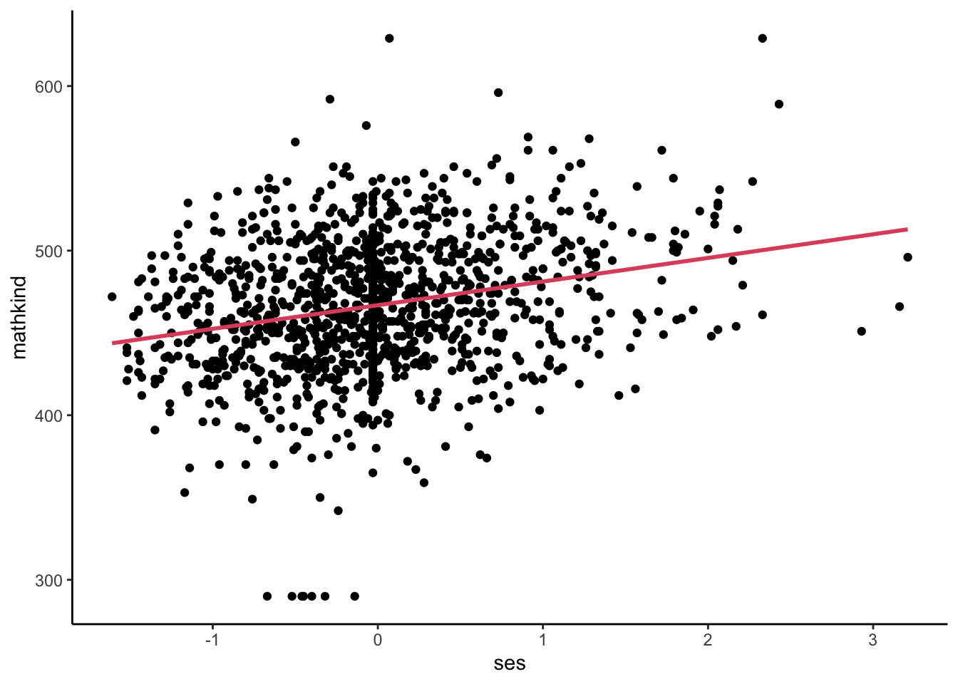
Code
- Numerically:
- Implicit: weight each student equally; assume independent observations
- Comparing two students differing by one unit of SES, we expect or predict a 14.4 unit difference in MATHKIND on average.
- Implicit: weight each student equally; assume independent observations
##
## Call:
## lm(formula = mathkind ~ ses, data = dat)
##
## Residuals:
##      Min       1Q   Median       3Q      Max
## -174.835  -26.399    1.065   26.529  161.150
##
## Coefficients:
##             Estimate Std. Error t value Pr(>|t|)
## (Intercept)  466.845      1.162  401.70   <2e-16 ***
## ses           14.359      1.568    9.16   <2e-16 ***
## ---
## Signif. codes:  0 '***' 0.001 '**' 0.01 '*' 0.05 '.' 0.1 ' ' 1
##
## Residual standard error: 40.08 on 1188 degrees of freedom
## Multiple R-squared:  0.06596,    Adjusted R-squared:  0.06518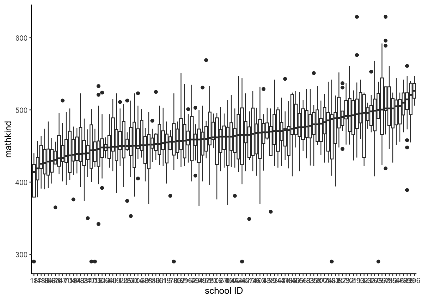
## F-statistic: 83.9 on 1 and 1188 DF, p-value: < 2.2e-16- We now examine the independence assumption with a simple descriptive exploration, the distribution of mathkind within schools using a stacked boxplot (x-axis is schoolid)
- We see some differences, at least in the median within school ()
- Why does this indicate non-independence within school? HINT: what would independence look like?
Code
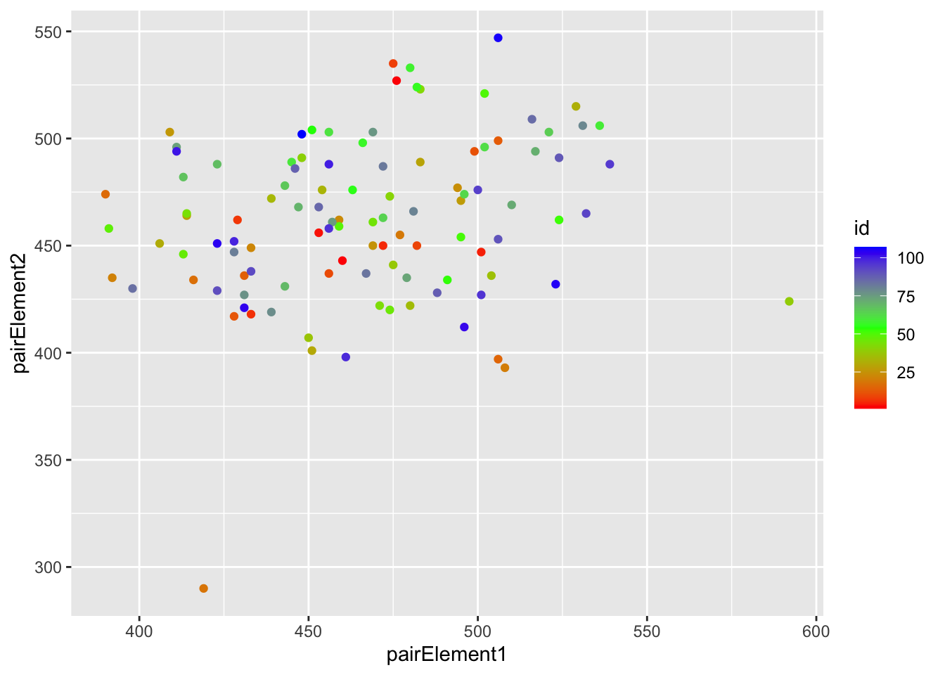
 v. Another way to examine dependence is to take a random draw of pairs of subjects within each school (repeating for all schools) and correlate the outcomes. If these have a significant correlation, then they are dependent.
a. When we do this, we get a correlation of about 0.23.
v. Another way to examine dependence is to take a random draw of pairs of subjects within each school (repeating for all schools) and correlate the outcomes. If these have a significant correlation, then they are dependent.
a. When we do this, we get a correlation of about 0.23.
Code
## [1] 0.2080421Code
- Some schools have higher outcomes, in general, but does the relationship between outcome and predictor vary by school (this is what we mean by a “response surface” for a predictor or set of them)?
- Here is an attempt to visualize some of the potential variation in the relationship of mathkind to ses by separately plotting the first 12 schoolids:
Code
## `geom_smooth()` using formula = 'y ~ x'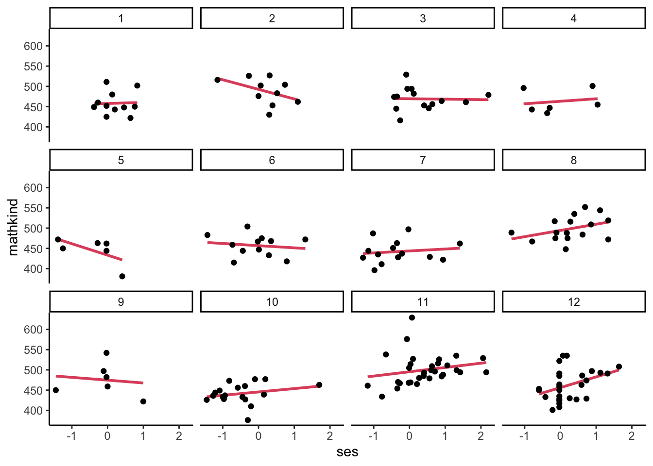
- The fitted lines are ‘mini-regressions,’ or ‘un-pooled’ regressions. What if we look at the coefficients from each of these? What might be a downside of doing this (is it practical to do this)? Would we get the same slope in each regression? How might we combine the school-specific slopes?
- One concern: small samples yield imprecise estimates
- Another concern: how to combine (meaningfully)?
- More subtle: do we want to assess the degree to which these slopes differ? Is this of intrinsic interest to us? (it may be)
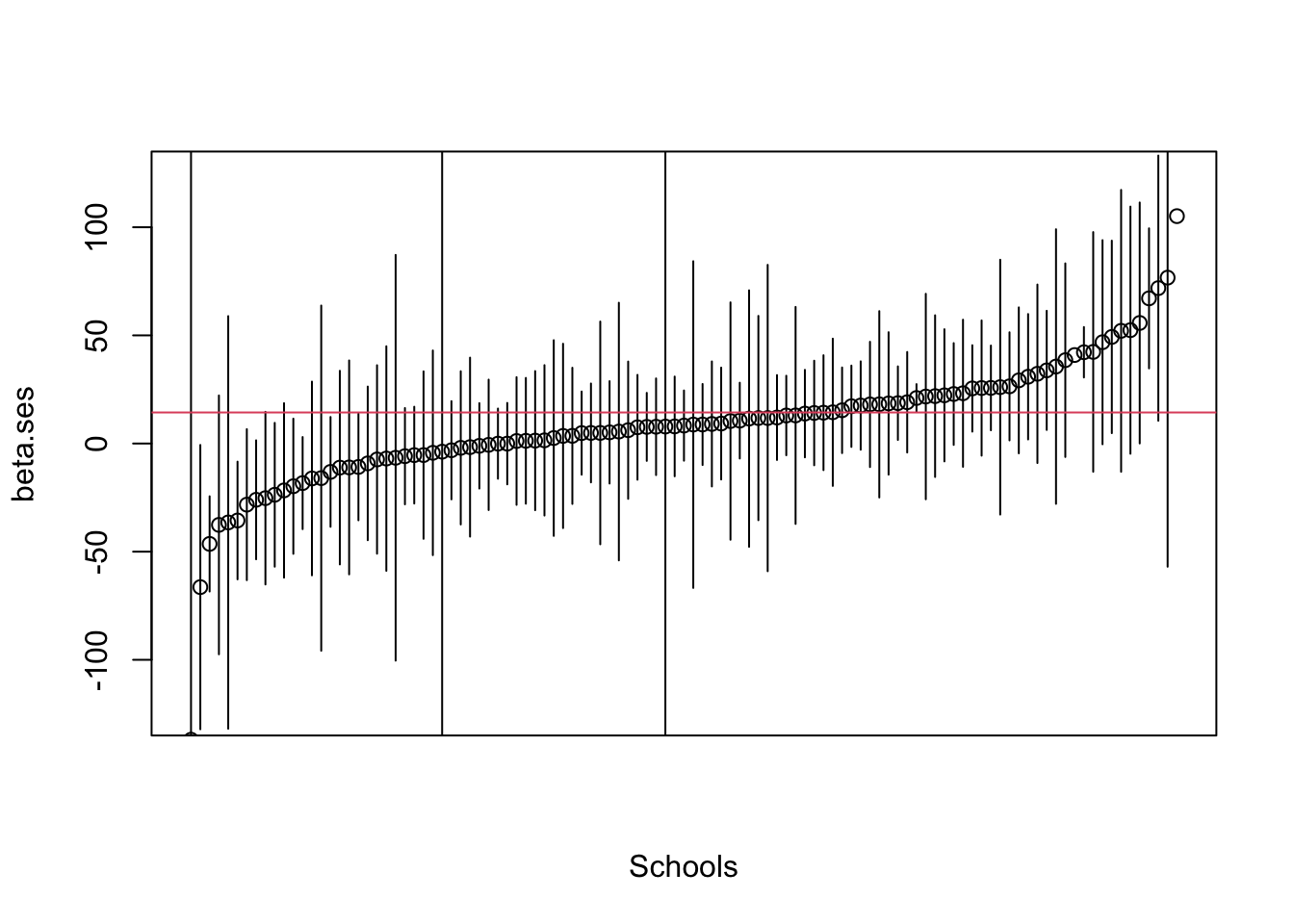
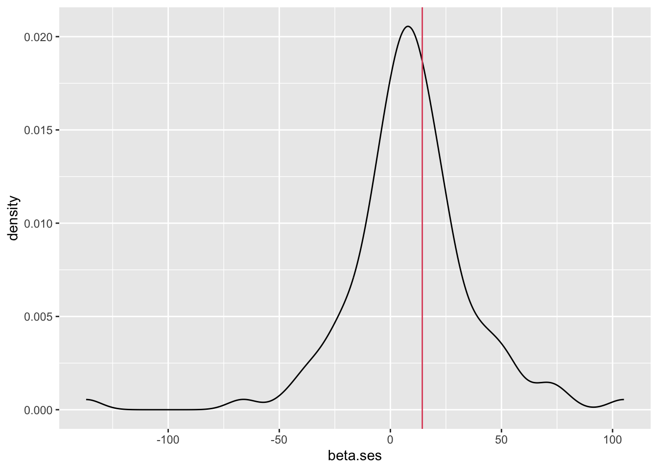
iii. Below are the coefficients (\(\hat\beta\)) from 107 separate regressions (one per school) of mathkind on ses. We plot these first in ascending order with 95% confidence bounds, then plot the density of the coefficients taken as an ensemble.
- The median in this ensemble of coefficients is 8.3, their mean is 8.6; a weighted mean is 10.3. Pooled (ignoring grouping) estimate is 14.4 (red line). Which one should you report?
- We follow the plot with the distribution of the coeffients. The range of school-level effects (the effect of SES) is substantial (mainly between -50 and 80).
Code
set.seed(2042001)
beta.ses <- 0
beta.se <- 0
school.n <- 0
idList <- unique(dat$schoolid)
len <- length(idList)
#slopes for SES by school, one for each.
for (i in 1:len) {
    b<-dat$schoolid==idList[i]
    school.n[i] <- sum(b)
    fit1<-lm(dat$mathkind[b]~dat$ses[b])
    beta.ses[i] <- fit1$coef[2]
    beta.se[i]<-summary(fit1)$coef[2,2]
}
#means using different weights:

#unweighted
wtd.beta1 <- mean(beta.ses)
print(wtd.beta1)
## [1] 8.6352## [1] 10.27034## Intercept X
## 466.84525 14.35929Code
Code
- This example shows us that we might need models that allow for:
- Correlation within groups
- Group-specific intercepts (level differences)
- Variation in the response (or “returns”) associated with a predictor on the outcome, by group. We eventually call these random slopes.
1.2 Modeling: first pass
- How can we write down a mathematical (statistical) model that accounts for some of this nested information, for our classroom example?
- The usual regression model, \(MATHKIND_i=b_0+b_1SES_i+\varepsilon_i\), in which the index \(i\) tracks the student to which we are referring, fails to capture anything about students being nested within schools. What if we added another subscripted index that tracked this?
- We write an equation: \(MATHKIND_{ij}=b_0+b_1SES_{ij}+\varepsilon_{ij}\). Notationally, \(MATHKIND_{ij}\) is the outcome for the \(i^{th}\) student in the \(j^{th}\) school, with corresponding predictor \(SES_{ij}\), and error \(\varepsilon_{ij}\).
- To uniquely identify a subject, we need both \(i\) and \(j\); this allows there to be more than one student indexed by \(i\) in two different schools.
- i.e., student identifiers should be thought of as pairs (student, school): (1,1), (2,1),…, (1,2),(2,2),… even if the actual IDs used in the dataset are unique across schools.
- Why go to this trouble of referring to schools in the subscript index? Because one way to account for the nested relationships is by introducing an “effect” indexed by group membership, and we need to associate effects with groups (here, schools).
- An effect is simply a way to account for a difference. At one extreme, we could model each school as having its own intercept – this is one type of effect. It could be implemented using indicator variables – one for each school (omitting a single reference school). This would involve 106 new parameters in our school example.
- If it is reasonable to assume that differences in level between schools (on average) follow a normal distribution and that we are not interested in specific levels for each school, but simply adjusting for those differences, then we can use a random effect to represent school (group) differences. With random effects:
- The assumption is that we have a sample from a population.
- We must also assume that these effects and errors are independent.
- Notationally, we use a Greek letter to represent a random effect and include enough indices to uniquely identify it:
\(MATHKIND_{ij} = b_0 + b_1SES_{ij} + \zeta_j + \varepsilon_{ij}\). School \(j\) gets a unique shift up or down, based on the value of \(\zeta_j\), its random effect. - There is more to do: There are two random (stochastic) components to the model and they must be further specified. We usually assume \(\zeta_j \sim N(0,\sigma_\zeta^2)\) [read this as, “zeta sub \(j\) is distributed as a normal random variable with mean 0 and variance sigma sub zeta squared] and \(\varepsilon_{ij} \sim N(0,\sigma_\varepsilon^2)\), independently of one another.
- To uniquely identify a subject, we need both \(i\) and \(j\); this allows there to be more than one student indexed by \(i\) in two different schools.
- With all of these components in place, we can fit the above model, \(MATHKIND_{ij} = b_0 + b_1SES_{ij} + \zeta_j + \varepsilon_{ij}\), using the method of maximum likelihood (this is what is commonly used in most statistical models you will encounter).
- One concern: what is the role of the \(\zeta_j\) term in the estimation? We do not plan to estimate each of these (107) separately, instead, we only estimate the variance of their distribution, \(\sigma_\zeta^2\).
- While we do not estimate them individually, they are still part of the model, so one can think of each subject in school \(j\) as having a school-specific intercept, \(\zeta_j\). Including the intercepts produces better estimates (in a manner to be made more precise) of the effects for the remaining predictors.
- While the error terms \(\varepsilon_{ij}\) are independent, outcomes are not, and this is our first attempt to capture this in a model. The way that we can quantify the dependence is by comparing observations within and between groups (here, indexed by \(j\)).
We find that under this model, the correlation between two outcomes is known precisely: \[ \mbox{Cor}(MATHKIND_{ij},MATHKIND_{i'j}) = \frac{\sigma_\zeta^2}{\sigma_\zeta^2 + \sigma_\varepsilon^2},\ \mbox{when}\ i\neq i' \]
- We assume \(j\) is the same (group or school) in this comparison. So observations are correlated in a prescribed manner, within schools.
\(Cor(MATHKIND_{ij},MATHKIND_{i'j'}) = 0,\ \mbox{when}\ j\neq j'\) (different groups, or schools in our example).
This is the proportion of variation between groups as a fraction of the total and also known as the Intraclass Correlation Coefficient (ICC).
- One concern: what is the role of the \(\zeta_j\) term in the estimation? We do not plan to estimate each of these (107) separately, instead, we only estimate the variance of their distribution, \(\sigma_\zeta^2\).
- Let’s fit the above model (more on ‘fitting’ near the end of class today) for our schools example.
- In R, there are two commonly used libraries for linear models with random effects: nlme and lme4. The lme4 library and corresponding
lmercommand will primarily be used in this course.lmer(mathkind~ses+(1|schoolid))is the syntax for a basic random intercept model.- The nested structure is specified inside parentheses and uses a vertical bar, ‘|’ to indicate the name of the grouping factor. The ‘1’ indicates a random intercept.
- The default fitting method is known as REML – we will discuss this later.
- Question: Do you have intuition for what a random effect is?
Code
## Linear mixed model fit by REML. t-tests use Satterthwaite's method [ ## lmerModLmerTest] ## Formula: mathkind ~ ses + (1 | schoolid) ## Data: dat ## ## REML criterion at convergence: 12038.7 ## ## Scaled residuals: ## Min 1Q Median 3Q Max ## -4.7423 -0.5716 0.0188 0.6343 3.7763 ## ## Random effects: ## Groups Name Variance Std.Dev. ## schoolid (Intercept) 309 17.58 ## Residual 1308 36.16 ## Number of obs: 1190, groups: schoolid, 107 ## ## Fixed effects: ## Estimate Std. Error df t value Pr(>|t|) ## (Intercept) 465.746 2.058 98.752 226.337 < 2e-16 *** ## ses 10.722 1.589 1187.995 6.747 2.35e-11 *** ## --- ## Signif. codes: 0 '***' 0.001 '**' 0.01 '*' 0.05 '.' 0.1 ' ' 1 ## ## Correlation of Fixed Effects: ## (Intr) ## ses 0.034## ANOVA-like table for random-effects: Single term deletions ## ## Model: ## mathkind ~ ses + (1 | schoolid) ## npar logLik AIC LRT Df Pr(>Chisq) ## <none> 4 -6019.3 12047 ## (1 | schoolid) 3 -6077.4 12161 116.1 1 < 2.2e-16 *** ## --- ## Signif. codes: 0 '***' 0.001 '**' 0.01 '*' 0.05 '.' 0.1 ' ' 1 - In R, there are two commonly used libraries for linear models with random effects: nlme and lme4. The lme4 library and corresponding
- Discussion of model fit results
- The components of this nested data model are divided into two sections.
- Random effects: listed as schoolid (intercept) is the estimated variance \(\hat{\sigma}^2_\zeta\) in level differences \(\zeta_j\) between schools. The value, 309, should be compared to the estimated residual variance, \(\hat{\sigma}_\varepsilon^2\), 1308.
- Fixed effects table (this label is controversial). The effect of a one unit change in SES on MATHKIND is 10.72, controlling for differences between schools, if our model and its assumptions are correct.
- The fraction of total variance accounted for by differences between groups is 309/(309+1308) = 0.19. This is also an estimate of the correlation between subjects within schools (and is the ICC).
- To know whether the random effects were ‘warranted’, we conduct a likelihood ratio (LR) test, as the model with and without the random effects are nested. The null tested is \(H_0: \sigma^2_\zeta=0\) using lmerTest package’s
randfunction.
a. The additional effects are warranted (p<.0001).
- The components of this nested data model are divided into two sections.
1.3 Simpler baseline models
- Some researchers prefer to start with simpler initial models. Typically, these include at least one random effect, but no predictors. This is called an unconditional means model (UMM).
- Why do it? It documents the extent to which variation appears to be between vs. within grouping factor(s).
- For school data, we can fit
\[
MATHKIND_{ij} = b_0 + \zeta_j + \varepsilon_{ij},\mbox{ with }\zeta_j\sim N(0,\sigma_\zeta^2), \varepsilon_{ij} \sim N(0,\sigma_\varepsilon^2),\mbox{ indep.}
\]
- Note: for those who are familiar with panel data models, clearly the UMM is more appropriate as a baseline model for nested data as contrasted to panel data (why?).
- Our lmer model simply drops the predictor SES, leaving:
lmer(mathkind~(1|schoolid))
## Linear mixed model fit by REML. t-tests use Satterthwaite's method [ ## lmerModLmerTest] ## Formula: mathkind ~ (1 | schoolid) ## Data: dat ## ## REML criterion at convergence: 12085.7 ## ## Scaled residuals: ## Min 1Q Median 3Q Max ## -4.8223 -0.5749 0.0005 0.6454 3.6237 ## ## Random effects: ## Groups Name Variance Std.Dev. ## schoolid (Intercept) 364.3 19.09 ## Residual 1344.5 36.67 ## Number of obs: 1190, groups: schoolid, 107 ## ## Fixed effects: ## Estimate Std. Error df t value Pr(>|t|) ## (Intercept) 465.23 2.19 103.20 212.4 <2e-16 *** ## --- ## Signif. codes: 0 '***' 0.001 '**' 0.01 '*' 0.05 '.' 0.1 ' ' 1## ANOVA-like table for random-effects: Single term deletions ## ## Model: ## mathkind ~ (1 | schoolid) ## npar logLik AIC LRT Df Pr(>Chisq) ## <none> 3 -6042.8 12092 ## (1 | schoolid) 2 -6119.3 12243 152.96 1 < 2.2e-16 *** ## --- ## Signif. codes: 0 '***' 0.001 '**' 0.01 '*' 0.05 '.' 0.1 ' ' 1- The fixed effects are uninteresting – simply a constant is reported.
- LR test indicates significant random effects (they are needed)
- The variances of the random effects are interesting. Using the formula
\(ICC=\frac{{\sigma_\zeta^2}}{{\sigma_\zeta^2 + \sigma_\varepsilon^2}}\), we see that 364.3/(364.3+1344.5)=21% of the variance is between schools (Reminder: ICC stands for intraclass correlation coefficient). This suggests that if we had school-level predictors, they might ‘explain’ some of this variation. Similarly, the 79% of the variation that is within schools might be explainable via student level (within-group) predictors.
- We have been focusing on schools as the grouping factor, but we have an even smaller grouping factor: classrooms. We can just as easily fit a model with groups determined by classrooms, which happen to be nested within schools.
- Three layers of nesting can be made explicit in the notation. Student \(i\) is in classroom \(j\) in school \(k\) (we had to ‘insert’ classroom before school, so the index for school becomes \(k\)). So one version of a model for outcomes is: \[ MATHKIND_{ijk} = b_0 + \eta_{jk} + \varepsilon_{ijk},\ \mbox{with}\ \eta_{jk} \sim N(0,\sigma_\eta^2)\ \mbox{and}\ \varepsilon_{ijk} \sim N(0,\sigma_\varepsilon^2);\ \mbox{with}\ \eta\perp\varepsilon \]
- In this model, the random effect associated with classrooms introduces a new symbol, \(\eta_{jk}\), to distinguish it from any school-level effects. The subscripts reflect the fact that classrooms are nested within schools. As before random effects and error are assumed independent of one another
- Notice that we have added an ‘extra’ index to the residual term).
- Notationally, we prefer to index classroom effects by \(jk\) because there could be two classrooms indexed by ‘\(j=1\)’ in two different schools (or just to organize the construction of effects). \(\eta_{jk}\) represents the effect for the \(j^{th}\) classroom in the \(k^{th}\) school.
- With lmer, we use the syntax:
lmer(mathkind~(1|classid))which indicates that there is a random intercept for the groups determined by classrooms (note that in this data, classid is unique between school as well. Had it not been, we would useschoolid:classidto refer to the unique index). The resulting fit is given next.
## Linear mixed model fit by REML. t-tests use Satterthwaite's method [ ## lmerModLmerTest] ## Formula: mathkind ~ (1 | classid) ## Data: dat ## ## REML criterion at convergence: 12149.4 ## ## Scaled residuals: ## Min 1Q Median 3Q Max ## -4.5541 -0.5719 -0.0173 0.6295 3.5807 ## ## Random effects: ## Groups Name Variance Std.Dev. ## classid (Intercept) 425.5 20.63 ## Residual 1305.8 36.14 ## Number of obs: 1190, groups: classid, 312 ## ## Fixed effects: ## Estimate Std. Error df t value Pr(>|t|) ## (Intercept) 465.866 1.629 272.864 285.9 <2e-16 *** ## --- ## Signif. codes: 0 '***' 0.001 '**' 0.01 '*' 0.05 '.' 0.1 ' ' 1## ANOVA-like table for random-effects: Single term deletions ## ## Model: ## mathkind ~ (1 | classid) ## npar logLik AIC LRT Df Pr(>Chisq) ## <none> 3 -6074.7 12155 ## (1 | classid) 2 -6119.3 12243 89.221 1 < 2.2e-16 *** ## --- ## Signif. codes: 0 '***' 0.001 '**' 0.01 '*' 0.05 '.' 0.1 ' ' 1- (cont.)
- The LR test indicates significant random effects for classrooms (this should not be surprising, since it was true for schools – why does this follow?)
- Using the formula \(ICC=\frac{{\sigma_\eta^2}}{{\sigma_\eta^2 + \sigma_\varepsilon^2}}\), we see that 425/(425+1306)=25% of the variance is between classrooms (ignoring schools).
- With more of the variance ‘explained’ by differences between classrooms, is this a better model (than the school-level model)? Perhaps, but this is not the way to make the assessment.
1.4 Two levels of nesting (schools and classrooms)
We now extend our example to include school-level effects in addition to the classroom level effects.
- The general outcome is \(Y_{ijk}\), for student \(i\) in classroom \(j\) in school \(k\).
- For now, we assume that there is only one observation per student (no repeated measures).
- We introduced notation that specifies effects for classrooms and schools separately, but their different names \(\eta_{jk},\zeta_k\) allow us to use them both in the same model. Notice how our random effects use just enough indices to be identifiable:
a. \(\zeta_k\) suffices for schools: we don’t need a classroom index, because all classrooms in school k will get this effect.
b. \(\eta_{jk}\) represents the effect for the \(j^{th}\) classroom in the \(k^{th}\) school; all students in that classroom will get this effect.
c. An unconditional means model for the outcome (no covariates), that includes effects for both schools and classrooms would then be specified as: \[Y_{ijk}=b_0+\eta_{jk}+\zeta_k+\varepsilon_{ijk}\]
d. Reminders: \(MATHKIND_{ijk}=Y_{ijk}\) in our example; The random effects \((\eta_{jk},\zeta_k)\) are taken as mutually independent and normally distributed, with level-specific variances, \(\sigma_\eta^2,\sigma_\zeta^2\), resp.; both are assumed independent of \(\varepsilon_{ijk}\) as well.- We write these distributional assumptions as: \(\eta_{jk}\sim N(0,\sigma_\eta^2)\), \(\zeta_{k}\sim N(0,\sigma_\zeta^2)\), independently of each other and \(\varepsilon_{ijk}\sim N(0,\sigma_\varepsilon^2)\).
We fit the model \(Y_{ijk}=b_0+\eta_{jk}+\zeta_k+\varepsilon_{ijk}\), in which schools and classrooms are modeled together. We interpret parameters in such a model as follows: net of school effects, how much additional systematic variation exists at the classroom level (in this case, level differences)?
- In the following R code, the order of the two random effects is important. Since classrooms are nested within schools, schoolid should be listed first.
- Failure to organize the nesting properly can result in a misspecified model – in this case, nesting schools within classrooms will generate more than one school effect for the same school, which is not correct.
- Note that two sets of group identifiers and a slightly different syntax is used.
- In computing the likelihood ratio test of significance for the random effects variance, the syntax changes as well.
## Linear mixed model fit by REML. t-tests use Satterthwaite's method [ ## lmerModLmerTest] ## Formula: mathkind ~ (1 | schoolid/classid) ## Data: dat ## ## REML criterion at convergence: 12085.1 ## ## Scaled residuals: ## Min 1Q Median 3Q Max ## -4.8198 -0.5749 0.0012 0.6303 3.5893 ## ## Random effects: ## Groups Name Variance Std.Dev. ## classid:schoolid (Intercept) 32.0 5.657 ## schoolid (Intercept) 352.8 18.784 ## Residual 1323.4 36.379 ## Number of obs: 1190, groups: classid:schoolid, 312; schoolid, 107 ## ## Fixed effects: ## Estimate Std. Error df t value Pr(>|t|) ## (Intercept) 465.220 2.191 103.579 212.4 <2e-16 *** ## --- ## Signif. codes: 0 '***' 0.001 '**' 0.01 '*' 0.05 '.' 0.1 ' ' 1Code
## Warning in anova.merMod(lme4, lm0, refit = F): some models fit with REML = ## TRUE, some not## Data: dat ## Models: ## lm0: mathkind ~ 1 ## lme4: mathkind ~ (1 | schoolid/classid) ## npar AIC BIC logLik deviance Chisq Df Pr(>Chisq) ## lm0 2 12245 12255 -6120.4 12241 ## lme4 4 12093 12113 -6042.5 12085 155.78 2 < 2.2e-16 *** ## --- ## Signif. codes: 0 '***' 0.001 '**' 0.01 '*' 0.05 '.' 0.1 ' ' 1- The estimated variances are: \(\hat{\sigma}^2_\eta=32.0;\ \hat{\sigma}^2_\zeta=352.8\).
- We can extend the formula for proportion of variance ‘explained’ by each effect. We simply include only one random effect variance at a time in the numerator, and sum all variance components in the denominator.
- So, 353/(353+32+1323), or about 21% of the variation is between schools, while 32/(353+32+1323), or 2% is between classrooms, net of schools; the remaining variation is within classrooms at the student level.
- Important: the last line of output gives an LR test that suggests that the model is improved significantly when both effects are included (as compared to linear regression).
We now add a covariate to the model \(Y_{ijk}=b_0+b_1SES_{ijk}+\eta_{jk}+\zeta_k+\varepsilon_{ijk}\), in which schools and classrooms are modeled together. We interpret the effect for that covariate as follows: net of school and classroom effects, what is the impact of a student’s SES on our outcome, MATHKIND?
## Linear mixed model fit by REML. t-tests use Satterthwaite's method [ ## lmerModLmerTest] ## Formula: mathkind ~ ses + (1 | schoolid/classid) ## Data: dat ## ## REML criterion at convergence: 12038.4 ## ## Scaled residuals: ## Min 1Q Median 3Q Max ## -4.7444 -0.5722 0.0112 0.6320 3.7507 ## ## Random effects: ## Groups Name Variance Std.Dev. ## classid:schoolid (Intercept) 20.44 4.521 ## schoolid (Intercept) 301.52 17.364 ## Residual 1294.08 35.973 ## Number of obs: 1190, groups: classid:schoolid, 312; schoolid, 107 ## ## Fixed effects: ## Estimate Std. Error df t value Pr(>|t|) ## (Intercept) 465.749 2.058 99.030 226.344 < 2e-16 *** ## ses 10.684 1.589 1187.053 6.725 2.72e-11 *** ## --- ## Signif. codes: 0 '***' 0.001 '**' 0.01 '*' 0.05 '.' 0.1 ' ' 1 ## ## Correlation of Fixed Effects: ## (Intr) ## ses 0.035Code
## Warning in anova.merMod(lme5, lm1, refit = F): some models fit with REML = ## TRUE, some not## Data: dat ## Models: ## lm1: mathkind ~ ses ## lme5: mathkind ~ ses + (1 | schoolid/classid) ## npar AIC BIC logLik deviance Chisq Df Pr(>Chisq) ## lm1 3 12166 12181 -6079.8 12160 ## lme5 5 12048 12074 -6019.2 12038 121.23 2 < 2.2e-16 *** ## --- ## Signif. codes: 0 '***' 0.001 '**' 0.01 '*' 0.05 '.' 0.1 ' ' 1- In terms of proportion of variation, 302/(302+20+1294), or about 19% of the total variation is between schools, while 20/(302+20+1294), or 1% is between classrooms, net of schools and SES; the remaining variation is within classrooms at the student level.
- The last lines give an LR test that suggests that the model is improved significantly when both effects are included. If you want to test the need for just one effect, such as \(\sigma^2_\eta\), you need another procedure.
- The estimate of \(\hat{\sigma}^2_\eta=20\), which is very small. We can ‘request’ confidence intervals as follows:
## Computing profile confidence intervals ...## 2.5 % 97.5 %
## .sig01 0.0000 114.8900
## .sig02 190.7281 446.5601
## .sigma 1179.5292 1418.8220- (cont.)
- (cont.)
- (cont.)
- But…confidence bounds for variance terms can never cross zero (conceptually, and estimation is constrained to prevent it), as variances are always positive.
- We need another way to test \(H_0:\sigma^2_\eta=0\).
- (cont.)
- To assess whether adding classroom effects, in addition to school effects is warranted, we do a likelihood ratio (LR) test comparing the a model without these effects to one that contains them. The models are nested, and the only difference between them is that in one, \(\sigma^2_\eta=0\), so the LR test will determine how unusual our results are, assuming this variance to be zero under the null. Sequentially:
a. We run the simpler model and store its estimates (this has already been done, as modellme1).
b. We run the more complex model and store its estimates (already done, as modellme5).
c. The LR test used theanovacommand (unless we specify refit=F, it automatically refits using ML not REML–to be explained in subsequent handouts).
d. Note that we show you two ways to attempt to derive this test. The first is direct (fit 2 nested models); the second derives multiple tests, and the ordering is such that it tests each random effect in the presence of the other, so we get the same result.
- (cont.)
## Data: dat
## Models:
## lme1: mathkind ~ ses + (1 | schoolid)
## lme5: mathkind ~ ses + (1 | schoolid/classid)
## npar AIC BIC logLik deviance Chisq Df Pr(>Chisq)
## lme1 4 12047 12067 -6019.3 12039
## lme5 5 12048 12074 -6019.2 12038 0.2565 1 0.6125## ANOVA-like table for random-effects: Single term deletions
##
## Model:
## mathkind ~ ses + (1 | classid:schoolid) + (1 | schoolid)
## npar logLik AIC LRT Df Pr(>Chisq)
## <none> 5 -6019.2 12048
## (1 | classid:schoolid) 4 -6019.3 12047 0.257 1 0.6125
## (1 | schoolid) 4 -6045.9 12100 53.359 1 2.778e-13 ***
## ---
## Signif. codes: 0 '***' 0.001 '**' 0.01 '*' 0.05 '.' 0.1 ' ' 1- (cont.)
- The p-value (0.61) suggests that we don’t need classroom level effects (we do not reject the null–Are you surprised?), but a “better” p-value divides this by 2 to reflect the evaluation on the boundary of the parameter space.1
1.5 Appendix
1.5.1 OLS & MLE (sketch)
- In this course, we rely exclusively on the theory associated with Maximum Likelihood Estimation (MLE) and you may not have been exposed to it very much (APSTA-GE.2122 delves into the details). These notes are an attempt to give you an idea of the method and contrast it to OLS, which you know from regression.
- Example: determining the mean of a population of known variance by examining a sample.
- This is a classic example. It seems easy – just take the mean of the sample, and you have a good estimate of the mean of the population from which it was derived, right? Yes, but why is this a good idea?
- There are certainly more complicated situations in which finding the “best” parameters isn’t straightforward… and you are in this situation in this course!
- To make progress with this concern, we have to make the assumptions more explicit. Let us say that we have a population of size N (very large) and we know that it is normally distributed with standard deviation one. We just don’t know the mean of this population, which we will call \(\mu\).
- We say that the data generating process (DGP) – the mechanism by which observations, X, are generated, is \(X\sim N(\mu,1)\) (a normal distribution with s.d.=1, so the variance is also 1).
- The probability of observing a single X from this distribution derives from the density:
\[f(X|\mu ) = \frac{1}{{\sqrt {2\pi } }}{e^{\frac{{ - {{(X - \mu )}^2}}}{2}}}\] This is called the density of X given \(\mu\) (so \(\mu\) is fixed); you can think of it as defining the shape of the histogram you would get if you sampled millions of observations of X (so you know which X values are more or less likely). Here is what it looks like for \(\mu=0\):
Code
set.seed(2042001) #normal mean example: #standard normal density displayed: grd <- seq(-4,4,length=9*100) plot(grd,dnorm(grd),type='l',xlab='X',ylab=expression(f(paste(X,"|",mu)))) dens <- density(rnorm(10000000)) x1 <- min(which(dens$x >= 2)) x2 <- max(which(dens$x < 5)) with(dens, polygon(x=c(x[c(x1,x1:x2,x2)]), y= c(0, y[x1:x2], 0), col="gray"))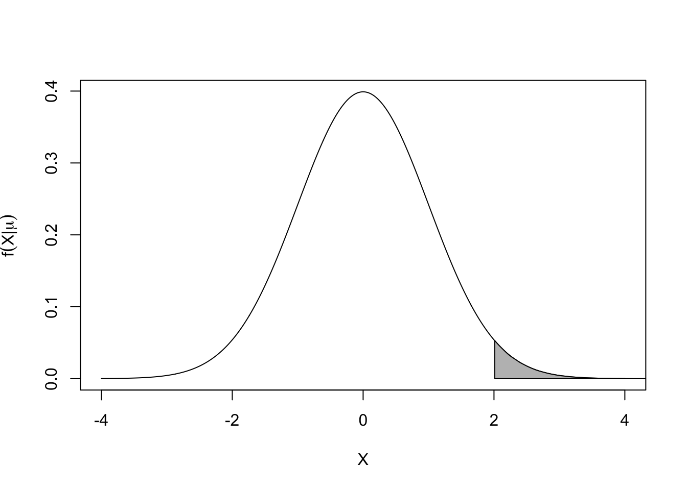
- (cont.)
- This is a familiar picture, and it allows you to calculate a probability. For example, P(X>2) is given by the shaded area under the curve. And X “near” 0 is most likely, while X “near” 4 is very unlikely.
- With a simple switch of the ordering, we define what we call the likelihood of \(\mu\) given X [this is different, conceptually]. \({\cal L}(\mu\vert X)=f(X\vert \mu)\). The conceptual difference is that we ask ourselves, which values of \(\mu\) are most likely to have given rise to the observed data, X (thus conditioning on X), assuming the model is correct?
- Example: determining the mean of a population of known variance by examining a sample.
- We can also evaluate the density of M multiple independent (standard normal) observations \((X_1,\ldots,X_M)\). It is:
\[ f({X_1},...,{X_M}|\mu ) = \prod\limits_{i = 1}^M {\frac{1}{{\sqrt {2\pi } }}{e^{\frac{{ - {{({X_i} - \mu )}^2}}}{2}}} = } \frac{1}{{{{(2\pi )}^{M/2}}}}{e^{\frac{{ - \sum\limits_{i = 1}^M {{{({X_i} - \mu )}^2}} }}{2}}} \] and the corresponding likelihood is \({\cal L}(\mu |{X_1},...,{X_M}) = f({X_1},...,{X_M}|\mu )\)
- In real situations, we observe \(X_1,\ldots,X_M\) and wish to infer \(\mu\). The principle of Maximum Likelihood says that we should choose \(\mu\) so that the log-likelihood, defined as
\(\ell(\mu |{X_1},...,{X_M}) = \log f({X_1},...,{X_M}|\mu ) = - \tfrac{M}{2}\log (2\pi ) - \tfrac{1}{2}\sum\limits_{i = 1}^M {{{({X_i} - \mu )}^2}}\)
is maximized (over the range of valid \(\mu\)).
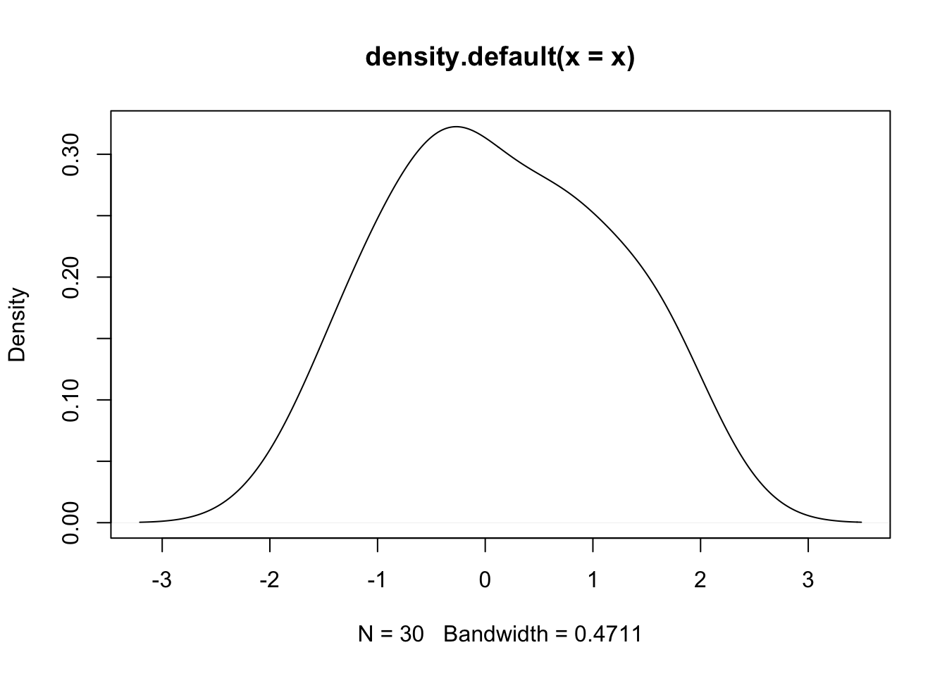
- Example (cont.): Say we have some number of independent observations, X, from a standard normal distribution, so the truth is that \(\mu=0\). Here is a density plot from a draw of 30:
- To apply the Principle of Maximum Likelihood, we calculate \(\ell(\mu |{X_1},...,{X_M}) = \log f({X_1},...,{X_M}|\mu )\) for a range of \(\mu\) and report the value that maximizes the log-likelihood \(\ell\). We did this for a grid of points between -4 and 4 and we get this plot.
Code
#set up for MLE: need the likelihood function (R codes this as dnorm): loglik.norm <- function(x,mu,sd=1) sum(dnorm(x,mean=mu,sd=sd,log=T)) #grid search - crude MLE grd <- seq(-4,4,length=9*10) ll <- rep(NA,length(grd)) #store loglik values here #compute ll across grid for (i in 1:length(grd)) ll[i] <- loglik.norm(x,mu=grd[i]) #plot ll across grid plot(grd,ll,type='p',pch=3,ylab='log-likelihood',xlab='proposed mu') lines(grd,ll,col=8) #connect the points abline(v=0,col=2) #true value of mu from population
- Clearly the choice of \(\mu\) that maximizes the log-likelihood is 0. It turns out that is also the mean of this sample (to a close approximation).
- You may have noticed that we were trying to find the \(\mu\) that maximizes:
\(-\tfrac{M}{2}\log (2\pi)-\tfrac{1}{2}\sum\limits_{i=1}^M{(X_i-\mu)^2}\)
and that since the first term is a constant, this will be a maximum when
\(\sum\limits_{i=1}^M{(X_i-\mu)^2}\) is minimized. There are lots of ways to find the minimum of that expression (those who know calculus should see that this quadratic is minimized at the sample mean), but for now, just notice that the expression looks a lot like the sum of squared residuals. The term “least squares” should come to mind.
- If you had a regression model (\(X\) as outcome) \(X_i = b_0 + \varepsilon_i\) with the usual assumptions of independent normal errors, then an OLS approach to finding an estimate \(\hat{b}_0\) would be to compute residuals from the model over different values of \(b_0\) and chose \(\hat{b}_0\) such that it minimizes the sum of squared residuals: \(\sum\limits_{i=1}^M{(X_i-b_0)^2}\). This should look familiar – it is the criterion used in the maximization of the log-likelihood, above, with \(b_0\) substituted for \(\mu\).
- For the estimation of unknown mean and known variance, the MLE and the OLS solution are identical and lead to optimizing with respect to the same sum of squares criterion.
- For the estimation of unknown mean and known variance, the MLE and the OLS solution are identical and lead to optimizing with respect to the same sum of squares criterion.
- Example 2: Poisson regression
- In this instance, OLS and MLE give different answers, and you would not “trust” the OLS results. We need to be clear, though, that by OLS, we mean applying a sum of squared residuals criterion to search for an “optimal” set of regression parameters.
- The model (for one explanatory predictor, and constant exposure) is:
\(\ln {\lambda_i} = {b_0} + {b_1}{X_i}\),
and \(Y_i\sim Pois(\lambda_i)\)
(Y is a Poisson random variable with rate \(\lambda_i\)).
Residuals from the model are of the form:\({Y_i} - \exp ({b_0} + {b_1}{X_i})\), where \(\exp(x)=e^x\).
- Using a likelihood-based approach, the density of Y (a count) follows a Poisson distribution:
\(f({Y_i}|{X_i},{b_0},{b_1}) = \frac{{{e^{ - {\lambda_i}}}{\lambda_i}^{{Y_i}}}}{{{Y_i}!}}\),
where \(\ln {\lambda_i} = {b_0} + {b_1}{X_i}\).
- When we extend this to M independent observations, the density becomes: \[ f({Y_1}, \ldots ,{Y_M}|{X_1}, \ldots ,{X_M},{b_0},{b_1}) = \frac{{{e^{ - {\lambda_1}}}{\lambda_1}^{{Y_i}}}}{{{Y_1}!}} \cdots \frac{{{e^{ - {\lambda_M}}}{\lambda_M}^{{Y_M}}}}{{{Y_M}!}} \] with \(\ln{\lambda_i}={b_0}+{b_1}{X_i}\ \mbox{for}\ i=1,\ldots,M\). Change \(X_i\) and you change the rate \(\lambda_i\).
- A likelihood based approach reverses this equation, so that you try to maximize (over \(b_0,b_1\)):
\[
{\cal L}({b_0},{b_1}|{X_1}, \ldots ,{X_M},{Y_1}, \ldots ,{Y_M}) = f({Y_1}, \ldots ,{Y_M}|{X_1}, \ldots ,{X_M},{b_0},{b_1})
\]
- You can imagine using a grid search through plausible \(b_0,b_1\) until you find one that maximizes that likelihood.
- The OLS approach would try to minimize \(\sum\limits_{i = 1}^M {{{({Y_i} - \exp ({b_0} + {b_1}{X_i}))}^2}}\) over plausible \(b_0,b_1\).
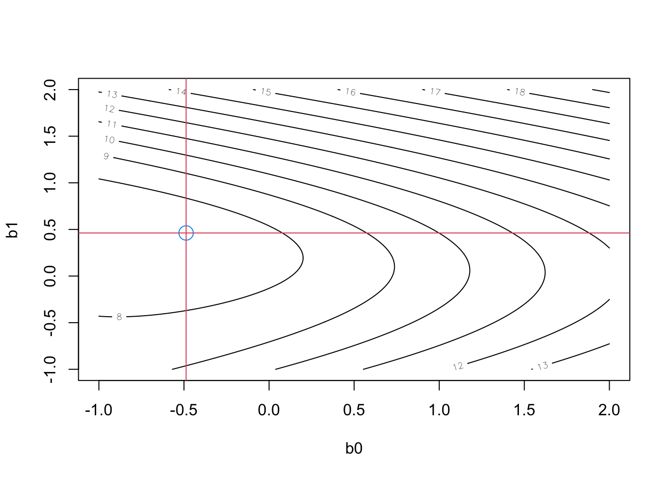
- We did a grid search over plausible \(b_0,b_1\) using this OLS approach, in which the true model was \(Y_i\sim Pois(\lambda_i)\), with \(\ln {\lambda_i} = - 0.5 + 0.5{X_i}\). We took a sample of size 3000, drawing X from a standard normal, and Y from a Poisson process, corresponding to the rates given by the “regression” portion of the model. We would hope to discover that \(\hat{b}_0=-0.5;\ \hat{b}_1=0.5\) (the truth).
- In our simulation, the OLS approach, minimizing sum of squared residuals, we get \(\hat{b}_0=-0.49;\ \hat{b}_1=0.46\). Here are some details:
Code
#poisson example set.seed(3) N<-3000 x <- rnorm(N) rt <- exp(-.5+.5*x) #model for poisson rate y <- rpois(N,rt) #generate data #use Sum Sqs criterion to search for best params in poisson model. this fn computes the sum sqs ssq.pois <- function(betas,x,y) { n <- dim(betas)[1] muhat <- betas%*%rbind(1,x) res <- matrix(rep(y,n),nrow=n,byrow=T) - exp(muhat) ssq <- apply(res*res,1,sum) ssq } #set up for grid search grd.len <- 4*5*10 #*2 for speedup grd <- seq(-1,2,length=grd.len) betas <- as.matrix(merge(grd,grd)) #trick to build the crossproduct of grid values in range (-1,2) for 2-D search ssq <- ssq.pois(betas,x,y) #this computes all 200*200 search points Sum Sqs rslts contour(x=grd,y=grd,z=ssq.mat<-matrix(log(ssq),grd.len,grd.len,byrow=F),xlab="b0",ylab="b1") min.loc <- which(ssq.mat==min(ssq.mat), arr.ind=T) cat("Grid-based fit (b0, b1): ",grd[min.loc])## Grid-based fit (b0, b1): -0.4874372 0.4623116Code
- The MLE approach yields this:
## ## Call: ## glm(formula = y ~ x, family = "poisson") ## ## Deviance Residuals: ## Min 1Q Median 3Q Max ## -2.3266 -1.0397 -0.7155 0.5440 3.4077 ## ## Coefficients: ## Estimate Std. Error z value Pr(>|z|) ## (Intercept) -0.50108 0.02456 -20.40 <2e-16 *** ## x 0.48534 0.02225 21.82 <2e-16 *** ## --- ## Signif. codes: 0 '***' 0.001 '**' 0.01 '*' 0.05 '.' 0.1 ' ' 1 ## ## (Dispersion parameter for poisson family taken to be 1) ## ## Null deviance: 3521.1 on 2999 degrees of freedom ## Residual deviance: 3042.7 on 2998 degrees of freedom ## AIC: 6206.9 ## ## Number of Fisher Scoring iterations: 5- The results are not terribly different, although with 3000 observations, one would expect to be able to recover the DGP parameters fairly precisely. And the MLE-based approach did get closer to the “truth.”
- But you must also ask yourself another question: if I use the result from OLS for Poisson regression, what are my confidence intervals for those estimates?
1.6 Coding
lsfit()lmer()rand()
lsfit()function is find a least square estimate of beta in the model \(Y = \beta X + \epsilon\) fromstatslibrary. It has arguments as follows:x: a matrix
y: the response (a matrix)
wt: an optional vectors of weights
intercept: whether of not an intercept term should be used
# A sample form of the function
lsfit(x, y, wt = NULL, intercept = TRUE,
tolerance = 1e-07, yname = NULL)
## Intercept         X
## 466.84525 14.35929lmer()function is to fit a linear mixed-effects model to data fromlme4library. It has arguments as follows:formula: A 2-sided linear formula object; Random-effects terms are distinguished by vertical bars (|) separating expressions for design matrices from grouping factors. Two vertical bars (||) can be used to specify multiple uncorrelated random effects for the same grouping variable.
data: a dataframe containing the variables in the formula
REML: logical scalar
Detail information can be found with a link: https://www.rdocumentation.org/packages/lme4/versions/1.1-29/topics/lmer
Code
## Linear mixed model fit by REML. t-tests use Satterthwaite's method ['lmerModLmerTest']
## Formula: Sepal.Length ~ Sepal.Width + (1 | Species)
## Data: iris
##
## REML criterion at convergence: 194.6
##
## Scaled residuals:
## Min 1Q Median 3Q Max
## -2.9846 -0.5842 -0.1182 0.4422 3.2267
##
## Random effects:
## Groups Name Variance Std.Dev.
## Species (Intercept) 1.0198 1.010
## Residual 0.1918 0.438
## Number of obs: 150, groups: Species, 3
##
## Fixed effects:
## Estimate Std. Error df t value Pr(>|t|)
## (Intercept) 3.4062 0.6683 3.4050 5.097 0.0107 *
## Sepal.Width 0.7972 0.1062 146.6648 7.506 5.45e-12 ***
## ---
## Signif. codes: 0 '***' 0.001 '**' 0.01 '*' 0.05 '.' 0.1 ' ' 1
##
## Correlation of Fixed Effects:
## (Intr)
## Sepal.Width -0.486rand()is a function to test likelihood ratio test (LRT) on random effects of linear mixed effects model fromlmerTestlibrary. It computes a Chi-square statistics and p-value of likelihood ratio tests as a data frame. It has arguments as follows:- model: linear mixed effects model
## ANOVA-like table for random-effects: Single term deletions
##
## Model:
## mathkind ~ ses + (1 | schoolid)
##                npar  logLik   AIC   LRT Df Pr(>Chisq)
## <none>            4 -6019.3 12047
## (1 | schoolid)    3 -6077.4 12161 116.1  1  < 2.2e-16 ***
## ---
## Signif. codes: 0 '***' 0.001 '**' 0.01 '*' 0.05 '.' 0.1 ' ' 11.7 Quiz
1.7.1 Self-Assessment
Use “W1 Activity Form” to submit your answers.
Selected questions will be discussed on Ed Discussion and you should fill out the first section of the corresponding google form with your answers.
Why are observations correlated, within schools?
If students were assigned to schools randomly – not based on where they live – would you expect much variation in average scores between schools?
Looking at the plot on p. 5. What does each dot represent? Explain why the order of the pair drawn for each school does not matter?
Understanding equations with ‘effects’: Rewrite the equation \(MATHKIND_{ij} = b_0 + b_1SES_{ij} + \zeta_j + \epsilon_{ij}\) in a slightly more familiar way. Here are the steps:
Replace the \(\zeta_j\) terms by a sum of indicator variables multiplied by the \(\zeta_j\) coefficients as follows: let \(D_j\) be \(1\) when person \(ij\) is in school \(j\) and zero otherwise; then there are \(D_1, D_2, …, D_J\) indicator variables, one for each of \(J\) schools.
Hint: the indicator for the 3rd school \((j=3)\) is \(D_3\) and the effect is \(\zeta_3\). Thus the term \(D_3\) will be equal to when \(\zeta_3\)*\(D_3 = 1\) and it is zero otherwise.
You need to replace \(\zeta_j\) in the above formula with a summation of terms similar to \(\zeta_3\)*\(D\) for \(j=1,...,J.\)
\[MATHKIND_{ij} = b_0 + b_1SES_{ij} + \sum_{j=1,2,...j}^{} \zeta_j D_j + \epsilon_{ij}\]
- If you ran a regression with all of those indicator variables, how many parameters would you have for “school effects”?
1.7.2 Lab Quiz
- Review the material in the Rshiny app “Week1: Handout1 Activity” and then answer these questions on the google form “W1 Activity Form”
1.7.3 Homework
- Homework is presented as the last section of the Rshiny app “Week1: Handout1 Activity”.
- Follow instructions there (fill out this form “W1 Activity Form” ) and hand in your code on Brightspace
We are of course assuming that treatment did not change the sex ratios.↩︎