Chapter 4 : BLUPs, Residuals, Information Criteria

4.1 Predicting Random Effects: BLUPs

Predicting the random effects after fitting a model: these predictions are known as BLUPs.
1. Why do this?
  1. We need to examine residuals that net out both fixed and random effects.
  2. We should look at estimates of the random effects themselves to check our model assumptions (they should be reasonably normally distributed).
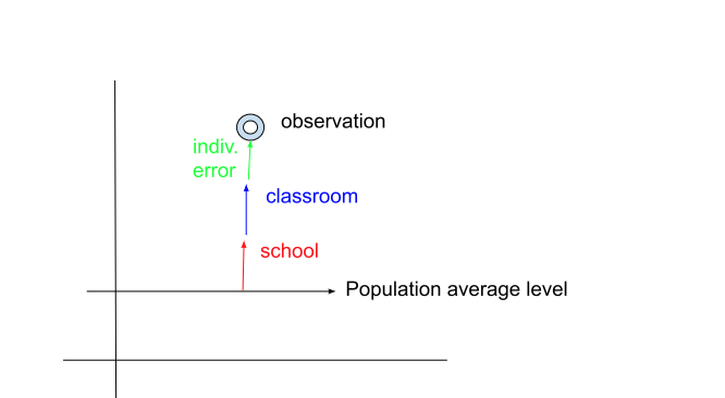
2. Consider a much simpler model: \[MATHGAIN_{ijk} = {b_0} + \zeta_k + \varepsilon_{ijk}, \mbox{ with }\zeta_k\sim N(0,\sigma_\zeta^2),\ \varepsilon_{ijk} \sim N(0,\sigma_\varepsilon^2), \mbox{indep.}\]
  1. In this two-level model, there are two types of errors: subject-level and group level, with these sometimes being referred to as level 1 and 2, \({\varepsilon_{ijk}}\) and \({\zeta_k}\), respectively.
  2. Residuals are estimates of these errors.
3. After fitting a model, we have an overall sense of the impact of the fixed and random effects, the latter of which are described by estimated variance components, such as \(\hat \sigma_\zeta^2\).
4. We can use the parameter estimates from the model fits, along with the observed outcomes and predictors to make a best guess – a prediction¹⁰ – as to where the \({\zeta_k}\) lie for each school k. Of course, this can be generalized in the presence of more fixed and random effects.
There is an explicit expression for ‘best guesses’ for \({\zeta_k}\). These are \[\hat\zeta_k = E(\zeta_k\vert Y_{\cdot k},X_{\cdot k}, \hat\beta,\hat\sigma_\zeta^2,\hat\sigma_\varepsilon^2),\] where \({Y_{\cdot k}}\) and \({X_{\cdot k}}\) denote all outcomes and predictors, respectively, associated with school \(k\).
1. In words, this is the conditional expectation (mean) of the random effect, \({\zeta_k}\), given the parameter estimates, the model, and the data relevant to school \(k\).
  1. Unconditionally, meaning in the absence of any additional information, the mean is zero; conditional on the observations and parameters, it is typically non-zero.
2. It is known as the Best Linear Unbiased Predictor, or BLUP, for the random effects, because it is the “best” guess under certain criteria.
3. We do not give the full formula for the BLUP (it requires matrix algebra), but we examine several of the simpler cases. The BLUP is a weighted average of what we might call ‘fixed effects residuals’ – the residuals we get after removing the population mean prediction.
  1. In our simple model, above, that would be \(MATHGAI{N_{ijk}} - {\hat b_0}\). In a model such as \(MATHGAI{N_{ijk}} = {b_0} + {b_1}SE{S_{ijk}} + {\zeta_k} + {\varepsilon_{ijk}}\), the corresponding fixed effects residual would be: \(MATHGAI{N_{ijk}} - ({\hat b_0} + {\hat b_1}SE{S_{ijk}})\)
  2. The weighted average combines only the relevant observations: those that are in the same school, in our example.
  3. The formula for a single school effect is: \[\hat \zeta_k\vert \hat e_{\cdot k},\hat\sigma_\zeta^2,\hat \sigma_\varepsilon^2 = \frac{\hat\sigma_\zeta^2}{\hat\sigma_\varepsilon^2 + n_k\hat\sigma_\zeta^2}\hat e_{\cdot k},\] where \(\hat e_{\cdot k} = \sum\limits_{i,j} (Y_{ijk} - X_{ijk}\hat\beta)\) is the sum of the residuals associated with school k, \(n_k\) is the number of subjects in that school and \(X_{ijk}\hat\beta\) is a shorthand for the prediction based on the fixed effects (you might be familiar with the term ‘y-hat’ used for such predictions. Y-hat is \({\hat b_0}\) in our model with a constant and \(\hat Y_{ijk} = \hat b_0 + \hat b_1 SES_{ijk}\) in our model with SES).
    iii.(cont.)
  1. The math symbol ‘\(\vert\)’ means “given,” so the left-hand side of the formula reads, “zeta sub k given e-hat sub dot k, sigma-hat-squared sub zeta, sigma-hat-squared sub epsilon”
  2. When \(\hat \sigma_\zeta^2\) is large compared to \(\hat\sigma_\varepsilon^2\), the formula reduces to approximately \(\frac{\hat\sigma_\zeta^2}{n_k\hat\sigma_\zeta^2}\hat e_{\cdot k} = \frac{1}{n_k}\hat e_{\cdot k}\), which is simply the mean residual – exactly what we calculated in a prior handout.
  3. When \(n_k=1\), we have no obvious way to disentangle the single residual into structured and unstructured components (but we have to). The formula simplifies, though, and assists us in this procedure:

\[ \hat \zeta_k|\hat e_{\cdot k},\hat \sigma_\zeta^2,\hat \sigma_\varepsilon^2 = \frac{\hat \sigma_\zeta^2}{\hat \sigma_\varepsilon^2 + \hat \sigma_\zeta^2}{\hat e_{\cdot k}} = IC{C_\zeta }{\hat e_{\cdot k}} \]

(cont.) iii.(cont.)
1. (cont.) + The ICC (associated with component \(\zeta\)) is a proportion between 0 and 1; the BLUP for the random effect is assigned as the ICC fraction of the residual for that case (the single residual is its own mean). + A large ICC implies that the residual should be more strongly apportioned to the random effect and vice versa. + This makes sense: if we don’t know how to partition a single observation into random effect and residual, we base the proportion on information from the full dataset (contained in the ICC). + When variance components \(\hat \sigma_\zeta^2\) and \(\hat \sigma_\varepsilon^2\) are equal, the ICC=0.5, so exactly half of the residual is taken as structured, and the other half is the remainder, or residual. Doesn’t this make intuitive sense?
2. When \(n_k\) is much greater than 1, \(\hat\sigma_\varepsilon^2\) will play a diminished role, as follows: + Imagine (relatively speaking) large error variance \(\hat\sigma_\varepsilon^2\approx 10\hat \sigma_\zeta^2\), which is what we’ve seen in the classroom data. ICC<0.10. Then if we have a lot of observations in each school, say n_k=100, we can predict school effects quite precisely, and \(\hat\sigma_\varepsilon^2\)’s effect on the BLUP will be inconsequential. + With a large within-group sample, the BLUP will tend to approach the value of the ‘fixed effects (average) residual’ for the school, since the fraction is approaching 1/n_k.
If the model is a bit more complicated, such as: \[ MATHGAIN_{ijk} = {b_0} + {\eta_{jk}} + {\zeta_k} + {\varepsilon_{ijk}}, \] \[ \mbox{ with } \varepsilon_{ijk}\sim N(0,\sigma_\varepsilon^2), \eta_{jk}\sim N(0,\sigma_\eta^2), \zeta_k\sim N(0,\sigma_\zeta^2), \mbox{ indep.}, \]

we can write an explicit expression for the BLUPs for a school k with one classroom j in it: \[ {\hat \eta_{jk}}\vert{\hat e_{\cdot k}},\hat \sigma_\eta^2,\hat \sigma_\zeta^2,\hat \sigma_\varepsilon^2 = \frac{{\hat \sigma_\eta^2}}{{\hat \sigma_\varepsilon^2 + {n_k}(\hat \sigma_\eta^2 + \hat \sigma_\zeta^2)}}{\hat e_{\cdot k}} \]

\[ {\hat \zeta_k}|{\hat e_{\cdot k}},\hat \sigma_\eta^2,\hat \sigma_\zeta^2,\hat \sigma_\varepsilon^2 = \frac{{\hat \sigma_\zeta^2}}{{\hat \sigma_\varepsilon^2 + {n_k}(\hat \sigma_\eta^2 + \hat \sigma_\zeta^2)}}{\hat e_{\cdot k}}, \]

where \(\hat e_{\cdot k} = \sum\limits_i (Y_{ijk} - X_{ijk}\hat\beta)\) is the sum of the residuals associated with school k (and thus classroom j in that school as well), n_k and \({X_{ijk}}\hat\beta\) are as before. i. Most of the comments from the prior example hold here as well. ii. When n_k = 1, we see that the three fractions: \[ \frac{\hat \sigma_\eta^2}{\hat \sigma_\varepsilon^2 + (\hat \sigma_\eta^2 + \hat \sigma_\zeta^2)},\ \frac{\hat \sigma_\zeta^2}{\hat \sigma_\varepsilon^2 + (\hat \sigma_\eta^2 + \hat \sigma_\zeta^2)}\ and \ \frac{\hat \sigma_\varepsilon^2}{\hat \sigma_\varepsilon^2 + (\hat \sigma_\eta^2 + \hat \sigma_\zeta^2)} \]

divide the ‘fixed effects residual’ (sum) into three parts, proportional to the variance of that component. 1. Since we are taking a residual and assigning portions of it to different types of error, it makes sense that if a specific unstructured error has the largest variance (relatively speaking), based on the model fit, then the largest portion of the residual should go to that component.
e. Matrix form (See Appendix)

Worked example: \[ MATHGAIN_{ijk} = {b_0} + {\zeta_k} + {\eta_{jk}} + {\varepsilon_{ijk}},\mbox{ with }\zeta_k\sim N(0,\sigma_\zeta^2),\ \eta_{jk}\sim N(0,\sigma_\eta^2)\ \varepsilon_{ijk} \sim N(0,\sigma_\varepsilon^2), \mbox{indep.} \]
1. R code for model fit and prediction of BLUPs (\({\hat \zeta_k}\),\({\hat \eta_{jk}}\)):

Code

fit2 <- lmer(mathgain~1+(1|schoolid/classid),data=dat)
print(summary(fit2))

## Linear mixed model fit by REML. t-tests use Satterthwaite's method ['lmerModLmerTest']
## Formula: mathgain ~ 1 + (1 | schoolid/classid)
##    Data: dat
## 
## REML criterion at convergence: 11768.8
## 
## Scaled residuals: 
##     Min      1Q  Median      3Q     Max 
## -4.6441 -0.5984 -0.0336  0.5334  5.6335 
## 
## Random effects:
##  Groups           Name        Variance Std.Dev.
##  classid:schoolid (Intercept)   99.22   9.961  
##  schoolid         (Intercept)   77.50   8.804  
##  Residual                     1028.23  32.066  
## Number of obs: 1190, groups:  classid:schoolid, 312; schoolid, 107
## 
## Fixed effects:
##             Estimate Std. Error     df t value Pr(>|t|)    
## (Intercept)   57.427      1.443 93.851   39.79   <2e-16 ***
## ---
## Signif. codes:  0 '***' 0.001 '**' 0.01 '*' 0.05 '.' 0.1 ' ' 1

Code

#generate BLUPs for random effs
ranefs <- ranef(fit2)
zetaM3 <- ranefs$schoolid[,1]
etaM3 <- ranefs$classid[,1]

#Alternative, using matrix alg.:
#reset classid to be 'in order'
Z <- cbind(model.matrix(~-1+factor(schoolid),data = dat), model.matrix(~-1+factor(classid),data = dat))
ehat <- dat$mathgain - predict(fit2,re.form=~0)
sig2.eta <- as.numeric(VarCorr(fit2))[1]  #retrieves squared vals.
sig2.zeta <- as.numeric(VarCorr(fit2))[2]  #retrieves squared vals.
sig2.eps <- sigma(fit2)^2
#construct  ZGZ'+I*sig.eps
nK <- length(unique(dat$schoolid))
nJ <- length(unique(dat$classid))
nI <- dim(dat)[1]
G <- diag(c(rep(sig2.zeta,nK),rep(sig2.eta,nJ)))
Sig <- Z%*%G%*%t(Z) + diag(rep(sig2.eps,nI)) 
Sig.inverse <- solve(Sig)
reffs <- G%*%t(Z)%*%Sig.inverse%*%ehat
zetaMatM3 <- reffs[1:nK]
etaMatM3 <- reffs[(nK+1):(nK+nJ)]
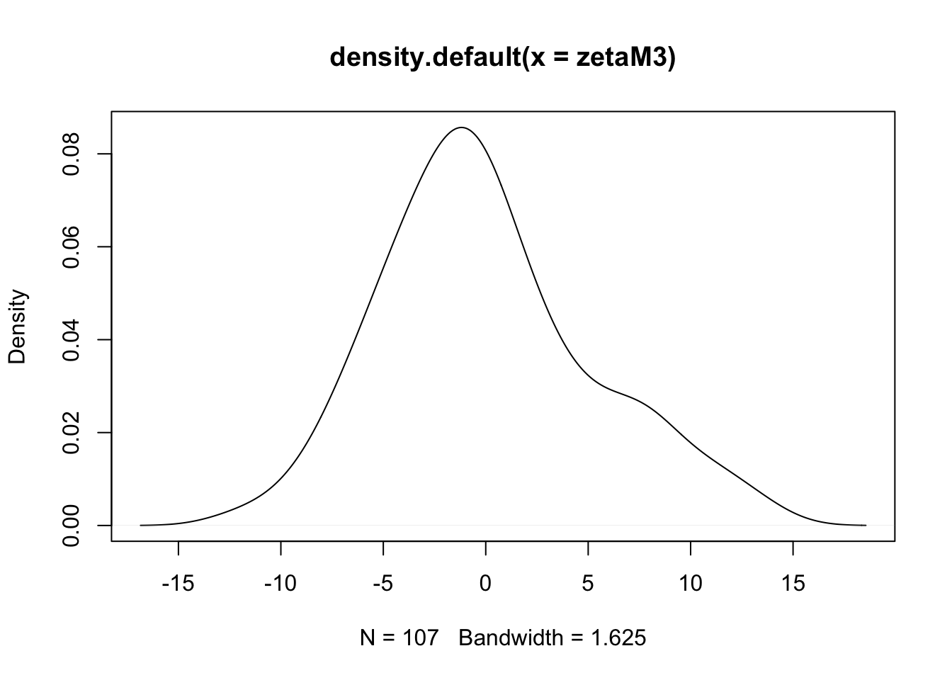
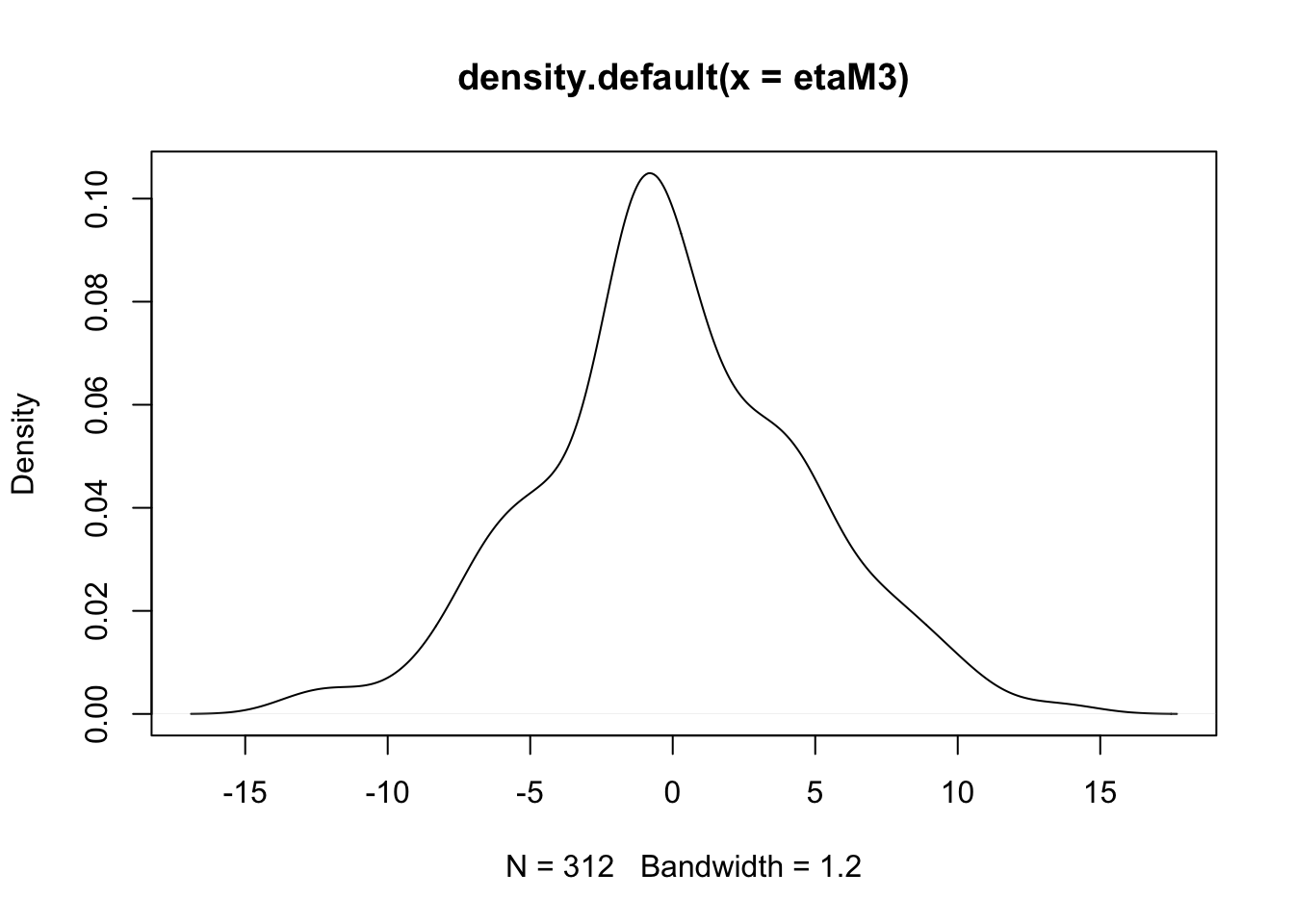
cor(zetaM3,zetaMatM3)

## [1] 1

Code

cor(etaM3,etaMatM3)

## [1] 1

(cont.)
1. If we wish to examine the BLUPs themselves, we need only ONE per school or classroom depending on the BLUP (in R, this was how the raw values were produced).

Code

#NOTE: R stores the data in vectors that don't have the replication problem
plot(density(zetaM3))

Code

qqnorm(zetaM3);qqline(zetaM3)

Code

plot(density(etaM3))

Code

qqnorm(etaM3);qqline(etaM3)

(cont.)
1. (cont.)
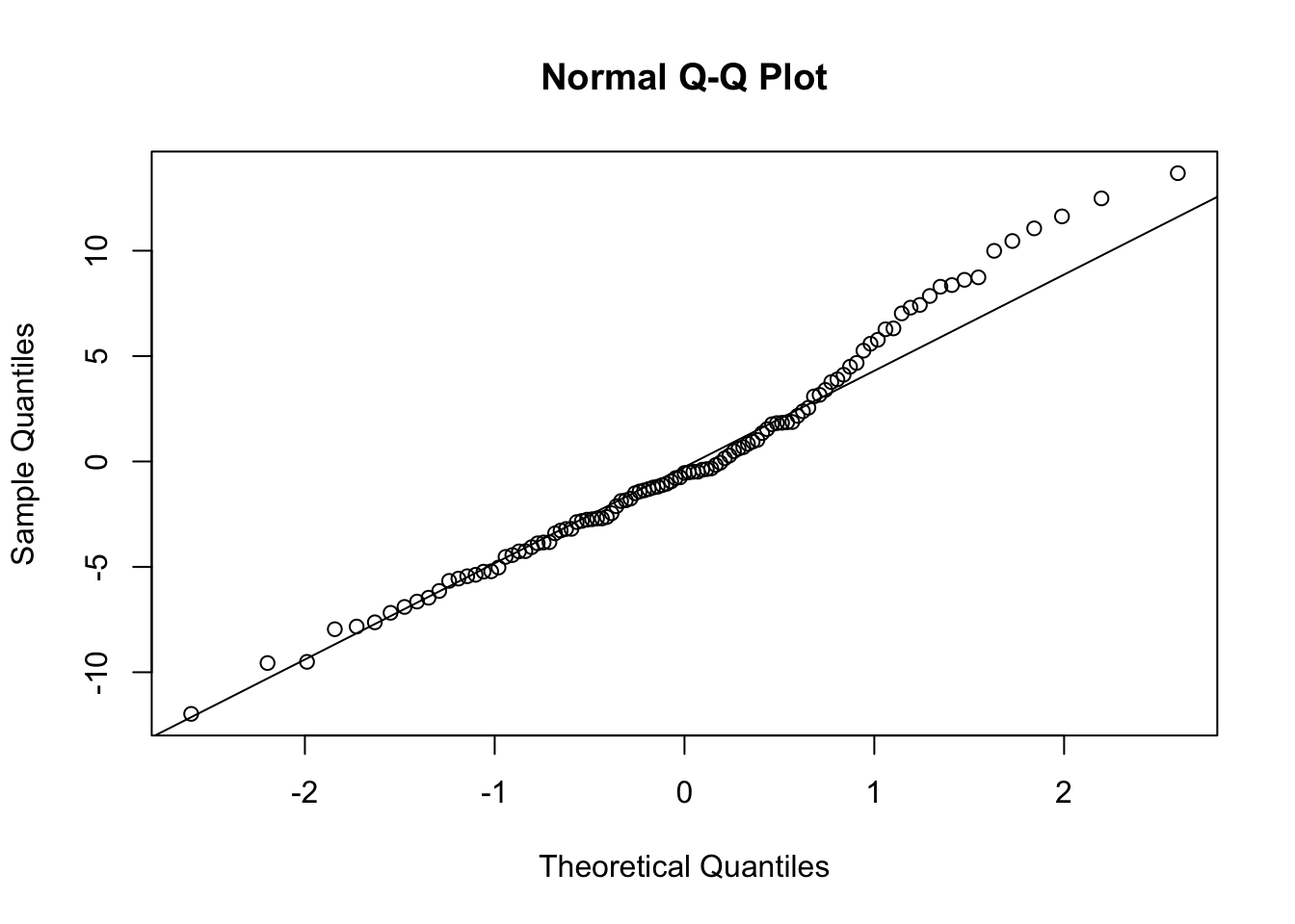
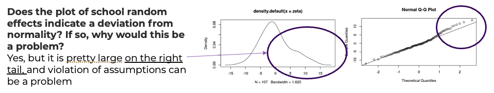
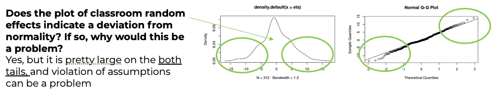
  1. There is some evidence of non-normality in the school effects, but it is probably tolerable (and sample is only 100 or so).
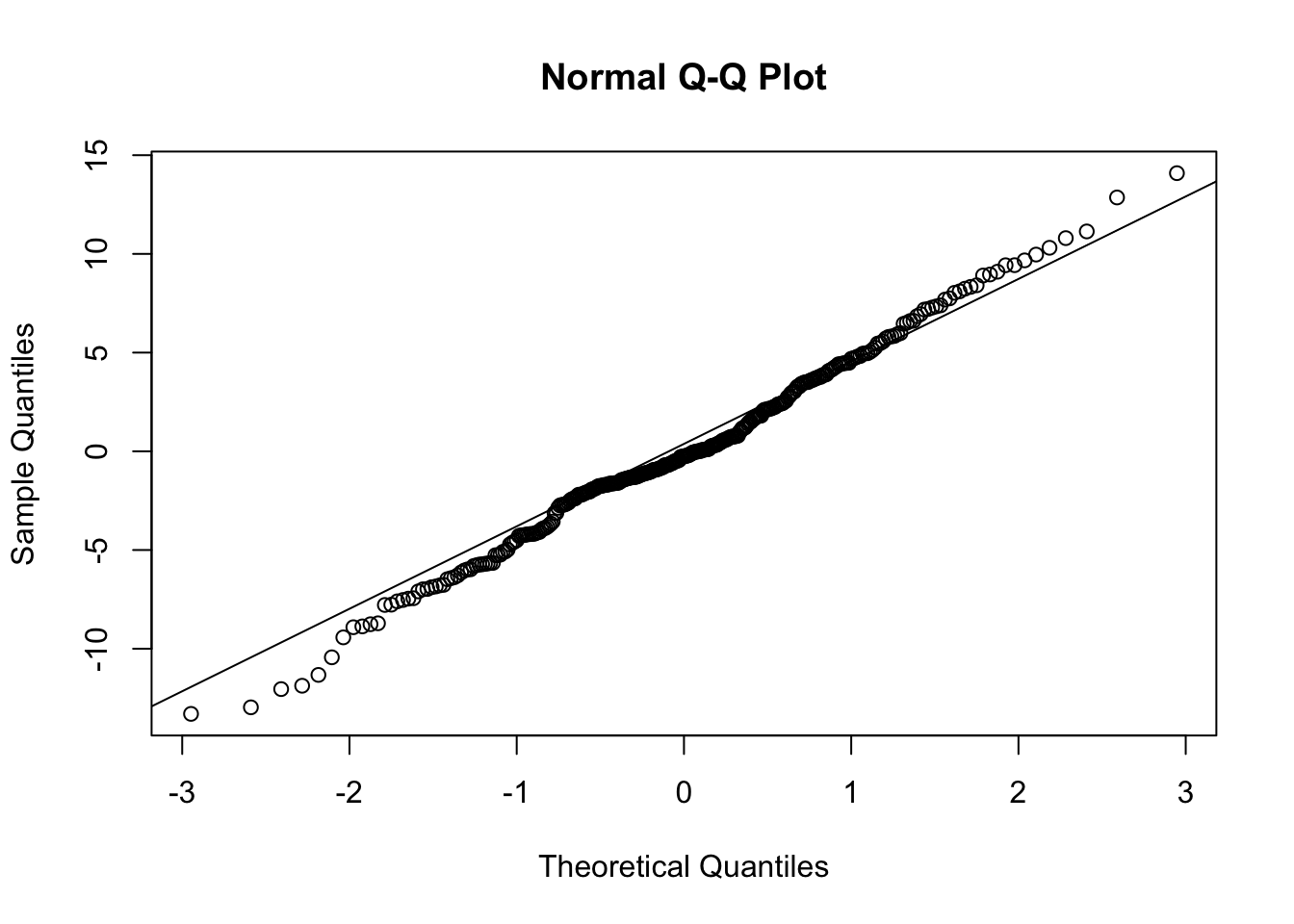
  2. It seems the BLUPs for classroom effects are a bit more normal, at least looking at the q-q plot, though the q-q plot shows some concern with the left tail.
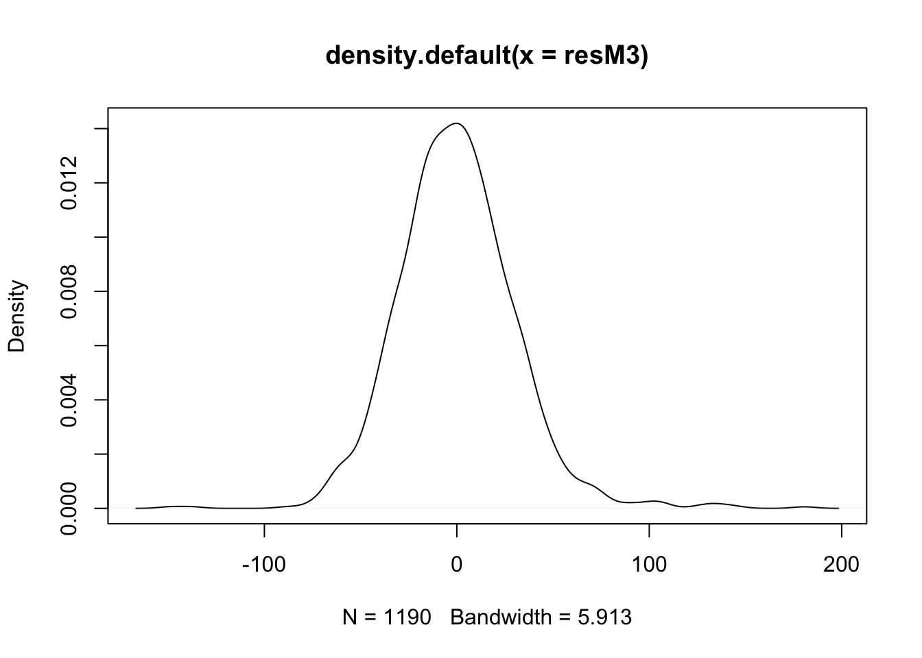
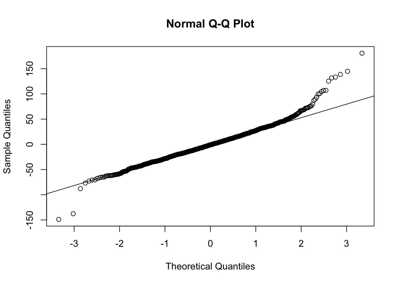
2. We often want to examine residuals based on the BLUPs (in other words, having netted out the random effects, or differences between schools and classrooms within them), and the next bit of code computes these directly from the model fit above.
  1. In the example, the estimate of the residual is: \({\hat \varepsilon_{ijk}} = MATHGAIN_{ijk} - ({b_0} + {\hat \zeta_k} + {\hat \eta_{jk}})\)
  2. If we examine the density & q-q plots of those residuals, it’s symmetric, but with heavier tails, especially the right tail.

Code

#*now residuals
#predict resM3, residual
resM3 <- residuals(fit2) #this has both school & classrm effects taken out
#kdensity resM3
plot(density(resM3))

Code

#qnorm resM3
qqnorm(resM3);qqline(resM3)

4.2 Examining residuals to uncover non-linearity

Just as in regression, residuals, particularly those associated with “level 1” or the subject level, are useful for uncovering non-linearity in the response to a covariate.
1. For this discussion, our baseline model will consist of one or two-layers of nesting (usually one) and we will add covariates to an unconditional means model: \[ Y_{ijk} = {b_0} + \zeta_k + \varepsilon_{ijk},\mbox{ with } \zeta_k\sim N(0,\sigma_\zeta^2), \varepsilon_{ijk}\sim N(0,\sigma_\varepsilon^2), \mbox{ indep.} \]

Code

fit.Mconst <- lmer(mathgain~1+(1|schoolid),data=dat,REML=F)

(cont.)
1. Residuals in an MLM can be constructed to reflect different ‘levels.’
  1. In a two-level model such as this, the BLUPs for \({\hat \zeta_k}\) can be understood as group-level (or level 2) residuals.
  2. The residuals most familiar to us, and the default residual produced by R/STATA, are those that net out the estimated fixed and random effects: subject level (or level 1) defined as follows:
    1. Given \({\hat b_0}\) and BLUP \({\hat \zeta_k}\), define a subject-level residual to be: \({\hat \varepsilon_{ijk}} = {Y_{ijk}} - ({\hat b_0} + {\hat \zeta_k})\).
  3. The R code to estimate these (after fitting a model) is given next. 1. Here, ‘resMconst’ is the name of the variable to which the residual is assigned.

Code

resMconst <- residuals(fit.Mconst)

(cont.)
1. (cont.)
  1. In some situations, it is useful to standardize the residuals in some manner.
    1. It can be especially important when searching for outliers by examining BLUPs for the random effects.
2. For this discussion, we do not standardize.
3. While we might examine the residuals marginally, looking at their distribution, and assessing normality, this is not the focus of this section.
4. It is good to examine the residuals grouped by categorical predictors, or in a scatterplot against a continuous predictor.
  1. Typically, we do this after including these in a model.
  2. When we do it before including them in a model, we are evaluating, qualitatively, whether we ‘need’ to include that predictor in the model, or trying to assess the likely functional form that would be required.
We use the residuals to explore the functional form for the fixed effects in what follows.
1. The predictor YEARSTEA (years teaching) was non-significant in some of the models we’ve examined. Could this have been an artifact of model misspecification?
  1. Examining the residuals from the model with just a constant (and thus every potential predictor omitted) plotted against some predictor in a scatterplot should reveal the functional form of that predictor. We will examine YEARSTEA.
  2. Use of a scatterplot smoother, such as ‘lowess,’ will help us assess the functional form.
    1. ‘Local’ smoothing functions can be understood as a running (weighted) mean of the outcome across different levels of a predictor. In this case it’s of the residual.
    2. The closest ‘crude’ way to construct a mean by predictor plot is to batch the predictor and display the mean or median for each batch. Stacked boxplots are a convenient approach.

Code

#*crude running mean:
#xtile icoso  = yearstea, nq(10)
dat$resMconst <- resMconst
dat$icoso <- with(dat, cut(yearstea,breaks=quantile(yearstea, probs=seq(0,1, by=0.10)),include.lowest=TRUE)) #this generates a factor
#graph box resMconst, over(icoso)
ggplot(dat, aes(x = icoso, y = resMconst)) + 
  geom_boxplot()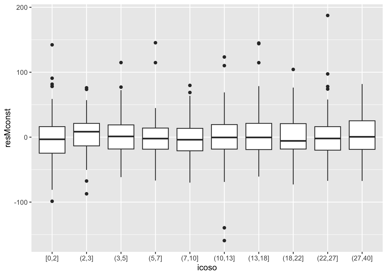

(cont.)

(cont.)
1. (cont.)
  1. (cont.)
    - This gives us a visualization of the median trend.
    - There may be a shift up in the first few years, but it’s hard to evaluate.
    - We don’t easily intuit the range of YEARSTEA on the x-axis. We use percentile based cut points above (each represents 5%).
  2. A better way to examine the mean at different levels of the predictor uses the lowess function (the code below merges a scatter plot with a ‘smooth’ line that captures the local trend).
    - We still cannot be sure of how ‘real’ the trend is, but we see a bump up at lower levels of teaching experience.
    - The magnitude of change is important. Even with this level of variability, a change from -10 to 0 could be about 0.3 s.d. (in terms of the residual), which is something.
    - We restrict the range of the residuals to +/- 100 to remove extreme outliers from this stage of the analysis.

Code

bool <- abs(dat$resMconst) < 100 #selection crit
ggplot(data=dat[bool,],aes(y=resMconst,x=yearstea))+
  geom_point()+
  stat_smooth(method="loess",span=.3,col=2)+
  geom_smooth(col=3,se=F)

## `geom_smooth()` using formula = 'y ~ x'
## `geom_smooth()` using method = 'gam' and formula = 'y ~ s(x, bs = "cs")'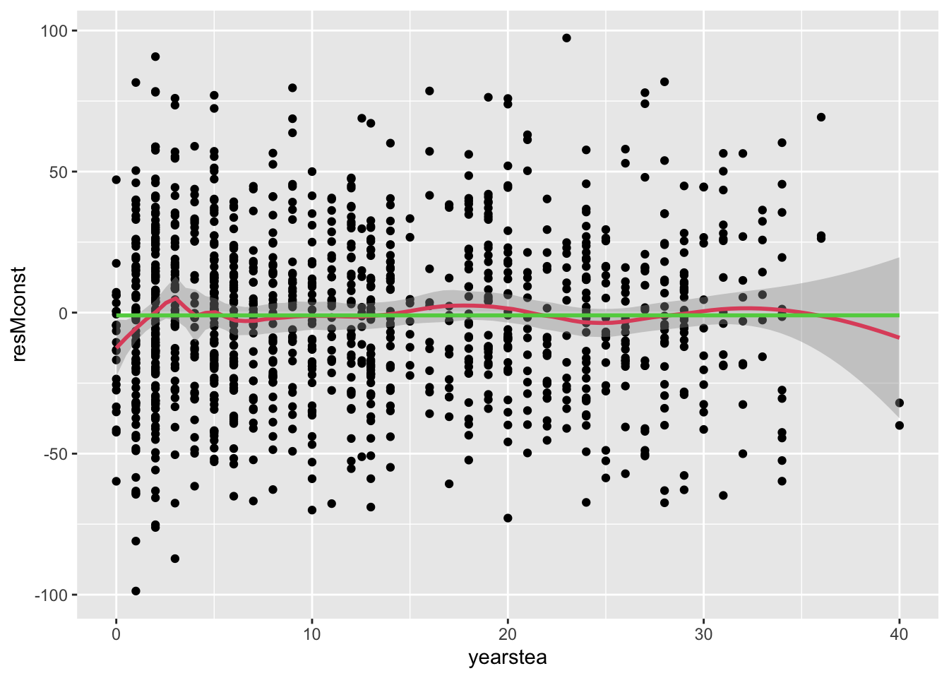

(cont.)
1. It seems reasonable to add a simple linear trend in YEARSTEA to the model and examine whether the residuals change very much. We don’t expect them to change, because the functional form we witness in the residuals, if it is real, looks non-linear. However, we should try.
  1. The new model is: \[ Y_{ijk} = b_0 + b_1 YEARSTEA_{jk} + \zeta_k + \varepsilon_{ijk},\mbox{ with }\zeta_k\sim N(0,\sigma_\zeta^2), \varepsilon_{ijk}\sim N(0,\sigma_\varepsilon^2) \mbox{ indep.} \]
  2. The corresponding R:

Code

fit.Mlin <- lmer(mathgain~yearstea+(1|schoolid),data=dat,REML=F)
print(summary(fit.Mlin))

## Linear mixed model fit by maximum likelihood . t-tests use Satterthwaite's method [lmerModLmerTest
## ]
## Formula: mathgain ~ yearstea + (1 | schoolid)
##    Data: dat
## 
##      AIC      BIC   logLik deviance df.resid 
##  11786.6  11806.9  -5889.3  11778.6     1186 
## 
## Scaled residuals: 
##     Min      1Q  Median      3Q     Max 
## -4.8065 -0.6018 -0.0134  0.5423  5.6328 
## 
## Random effects:
##  Groups   Name        Variance Std.Dev.
##  schoolid (Intercept)  106.5   10.32   
##  Residual             1093.7   33.07   
## Number of obs: 1190, groups:  schoolid, 107
## 
## Fixed effects:
##              Estimate Std. Error        df t value Pr(>|t|)    
## (Intercept)  56.42873    2.00212 228.17769  28.184   <2e-16 ***
## yearstea      0.09391    0.11357 864.77209   0.827    0.409    
## ---
## Signif. codes:  0 '***' 0.001 '**' 0.01 '*' 0.05 '.' 0.1 ' ' 1
## 
## Correlation of Fixed Effects:
##          (Intr)
## yearstea -0.699

(cont.)
1. (cont.)
  1. Note that the parameter estimate is not significant. This in itself suggests that the residuals won’t change much, but we explore this further for completeness.

Code

#predict residuals
resMlin <- residuals(fit.Mlin)
dat$resMlin <- resMlin
#plot the scatter & smooth
bool <- abs(dat$resMlin) < 100 #selection crit
ggplot(data=dat[bool,],aes(y=resMlin,x=yearstea))+
  geom_point()+
  stat_smooth(method="loess",span=.3,col=2)+
  geom_smooth(col=3,se=F)

## `geom_smooth()` using formula = 'y ~ x'
## `geom_smooth()` using method = 'gam' and formula = 'y ~ s(x, bs = "cs")'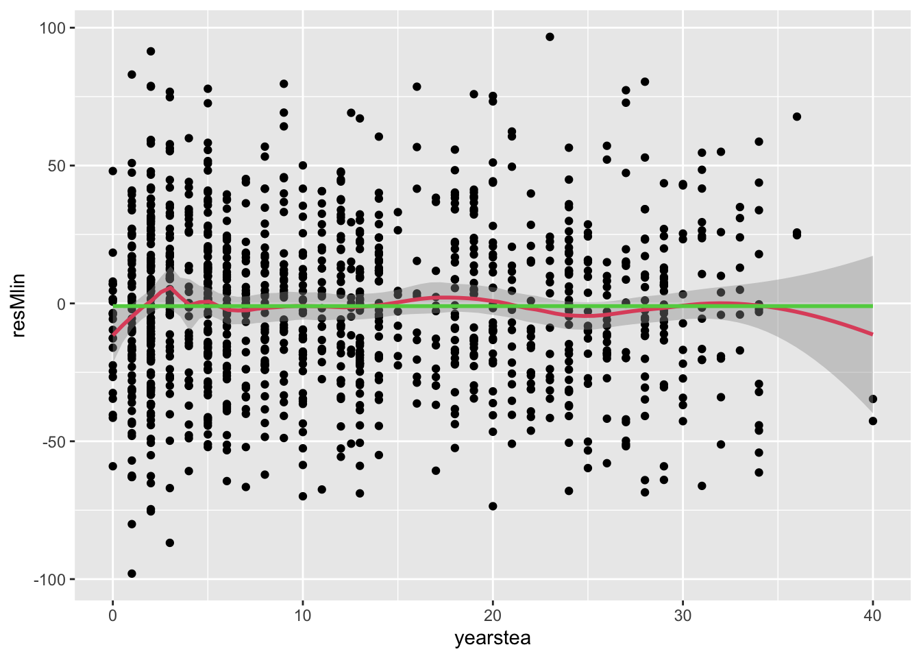

(cont.)
1. (cont.)
1. (cont.) 1. As expected, very little changed.
2. In what follows, we try many different functional forms to understand the relationship between YEARSTEA and MATHGAIN. Perhaps we ‘dig’ a bit more than I’d recommend, in general. However, the approach is illustrative of the potential gains one can achieve when one is willing to utilize more flexible forms for mean processes.
A first, reasonable approach to modeling a non-linear process is to include indicator variables that represent different levels of the predictor.

This is sometimes called a non-parametric approach, because it does not fix the functional form to be linear or nearly linear – it will reflect structure suggested by the data.
R has a fairly easy way to construct equal-sized bins for any variable. The cut command generates a factor variable whose levels reflect the number of quantiles chosen.
1. We will choose five equal group sizes, known as quintiles. The corresponding model is (with first quintile omitted).
  \[ Y_{ijk} = b_0+b_2 IQUINT2_{jk}+b_3 IQUINT3_{jk} +b_4 IQUINT4_{jk}+b_5 IQUINT5_{jk}+\zeta_k+\varepsilon_{ijk} \]

b.(cont.) i. (cont.) where IQUINTn is the indicator for the \(n^{th}\) quintile of YEARSTEA, and \({\zeta_k} \sim N(0,\sigma_\zeta^2)\), \({\varepsilon_{ijk}} \sim N(0,\sigma_\varepsilon^2)\) independent of one another. ii. We do an LRT test on \({H_0}:{b_2} = {b_3} = {b_4} = {b_5} = 0\) (the corresponding Wald test is slightly different and was described at the end of Handout 3).

```r
#*try dummy variables
dat$quint <- with(dat, cut(yearstea,breaks=quantile(yearstea, probs=seq(0,1, by=0.20)),include.lowest=TRUE)) #this generates a factor
fit.Mquint <- lmer(mathgain~quint+(1|schoolid),data=dat,REML=F)
print(summary(fit.Mquint))
```

```
## Linear mixed model fit by maximum likelihood . t-tests use Satterthwaite's method [lmerModLmerTest
## ]
## Formula: mathgain ~ quint + (1 | schoolid)
##    Data: dat
## 
##      AIC      BIC   logLik deviance df.resid 
##  11788.9  11824.5  -5887.4  11774.9     1183 
## 
## Scaled residuals: 
##     Min      1Q  Median      3Q     Max 
## -4.7617 -0.5921 -0.0228  0.5507  5.6567 
## 
## Random effects:
##  Groups   Name        Variance Std.Dev.
##  schoolid (Intercept)  103.1   10.15   
##  Residual             1091.7   33.04   
## Number of obs: 1190, groups:  schoolid, 107
## 
## Fixed effects:
##              Estimate Std. Error       df t value Pr(>|t|)    
## (Intercept)   55.9448     2.4574 319.5584  22.766   <2e-16 ***
## quint(3,7]     2.0954     3.3141 937.8890   0.632   0.5274    
## quint(7,13]   -0.7103     3.4176 576.7401  -0.208   0.8354    
## quint(13,22]   5.9192     3.4309 851.2444   1.725   0.0848 .  
## quint(22,40]   1.9517     3.3690 778.2808   0.579   0.5625    
## ---
## Signif. codes:  0 '***' 0.001 '**' 0.01 '*' 0.05 '.' 0.1 ' ' 1
## 
## Correlation of Fixed Effects:
##             (Intr) q(3,7] q(7,13 q(13,2
## quint(3,7]  -0.614                     
## quint(7,13] -0.653  0.459              
## qunt(13,22] -0.616  0.452  0.472       
## qunt(22,40] -0.637  0.451  0.481  0.457
```

```r
#LRT
anova(fit.Mconst,fit.Mquint,refit=F)
```

```
## Data: dat
## Models:
## fit.Mconst: mathgain ~ 1 + (1 | schoolid)
## fit.Mquint: mathgain ~ quint + (1 | schoolid)
##            npar   AIC   BIC  logLik deviance  Chisq Df Pr(>Chisq)
## fit.Mconst    3 11785 11800 -5889.6    11779                     
## fit.Mquint    7 11789 11824 -5887.4    11775 4.3553  4     0.3601
```

(cont.)
1. (cont.)
  1. Non-significant finding, so the data are consistent with no level shifts across the five equally-sized levels of YEARSTEA (maybe you were thinking that Iquint4, with \(p\approx .08\), would lead the batch of coefficients to significance?).
  2. We could try deciles, or even larger numbers of quantiles, but it is unlikely that we have enough data to support too many levels (try it at home).
2. We now examine residuals graphically to see whether these quintile-based means, while non-significant, are at least changing the patterns in the residuals. 1. Comment: we see very little change with the exception of the bump near 18 or 20 years of experience shrinking.

Code

resMquint <- residuals(fit.Mquint)
dat$resMquint <- resMquint
bool <- abs(dat$resMquint) < 100 #selection crit
ggplot(data=dat[bool,],aes(y=resMquint,x=yearstea))+
  geom_point()+
  stat_smooth(method="loess",span=.3,col=2)+
  geom_smooth(col=3,se=F)

## `geom_smooth()` using formula = 'y ~ x'
## `geom_smooth()` using method = 'gam' and formula = 'y ~ s(x, bs = "cs")'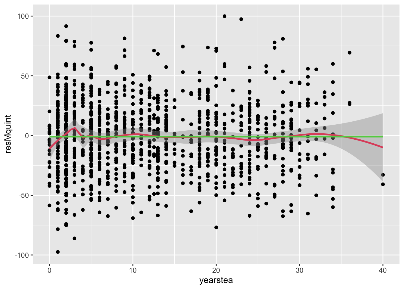

3. It is worth considering, for completeness, a polynomial functional form. These are relatively easy to specify and test. a. Given the residuals from the unconditional means model, we should at least consider a model with cubic terms for YEARSTEA:
\[ Y_{ijk} = b_0 + b_1 YEARSTEA_{jk} + b_2 YEARSTEA_{jk}^2 + b_3 YEARSTEA_{jk}^3 + \zeta_k + \varepsilon_{ijk}, \] \[ \mbox{ with }\zeta_k\sim N(0,\sigma_\zeta^2),\varepsilon_{ijk}\sim N(0,\sigma_\varepsilon^2),\mbox{ indep.} \] 3. (cont.) b. The code and results, including LR test:

Code

#*try cubic
#NOTE: R can do this without adding new vars to the dataset using I()
fit.Mcubic <-lmer(mathgain~yearstea+I(yearstea^2)+I(yearstea^3)+(1|schoolid),data=dat,REML=F)

## Warning: Some predictor variables are on very different scales: consider rescaling

## Warning: Some predictor variables are on very different scales: consider rescaling

Code

print(summary(fit.Mcubic))

## Linear mixed model fit by maximum likelihood . t-tests use Satterthwaite's method [lmerModLmerTest
## ]
## Formula: mathgain ~ yearstea + I(yearstea^2) + I(yearstea^3) + (1 | schoolid)
##    Data: dat
## 
##      AIC      BIC   logLik deviance df.resid 
##  11789.3  11819.8  -5888.7  11777.3     1184 
## 
## Scaled residuals: 
##     Min      1Q  Median      3Q     Max 
## -4.8577 -0.5925 -0.0223  0.5453  5.6395 
## 
## Random effects:
##  Groups   Name        Variance Std.Dev.
##  schoolid (Intercept)  108.2   10.40   
##  Residual             1091.7   33.04   
## Number of obs: 1190, groups:  schoolid, 107
## 
## Fixed effects:
##                 Estimate Std. Error         df t value Pr(>|t|)    
## (Intercept)    5.366e+01  3.298e+00  4.867e+02  16.270   <2e-16 ***
## yearstea       9.213e-01  9.047e-01  8.528e+02   1.018    0.309    
## I(yearstea^2) -4.704e-02  6.459e-02  8.908e+02  -0.728    0.467    
## I(yearstea^3)  6.967e-04  1.287e-03  9.041e+02   0.541    0.588    
## ---
## Signif. codes:  0 '***' 0.001 '**' 0.01 '*' 0.05 '.' 0.1 ' ' 1
## 
## Correlation of Fixed Effects:
##             (Intr) yearst I(y^2)
## yearstea    -0.813              
## I(yearst^2)  0.687 -0.959       
## I(yearst^3) -0.592  0.887 -0.979
## fit warnings:
## Some predictor variables are on very different scales: consider rescaling

Code

#joint test: yearstea yearstea_sq yearstea_cu
anova(fit.Mconst,fit.Mcubic,refit=F)

## Data: dat
## Models:
## fit.Mconst: mathgain ~ 1 + (1 | schoolid)
## fit.Mcubic: mathgain ~ yearstea + I(yearstea^2) + I(yearstea^3) + (1 | schoolid)
##            npar   AIC   BIC  logLik deviance  Chisq Df Pr(>Chisq)
## fit.Mconst    3 11785 11800 -5889.6    11779                     
## fit.Mcubic    6 11789 11820 -5888.7    11777 1.9311  3     0.5868

(cont.)
1. (cont.)
  1. It is not significant, suggesting again that there is no effect of YEARSTEA on the MATHGAIN outcome. Not even a cubic functional form.
  2. Examining residuals once more, we see no explanatory power in this cubic YEARSTEA specification:

Code

resMcubic <- residuals(fit.Mcubic)
dat$resMcubic <- resMcubic
bool <- abs(dat$resMcubic) < 100 #selection crit

ggplot(data=dat[bool,],aes(y=resMcubic,x=yearstea))+
  geom_point()+
  stat_smooth(method="loess",span=.3,col=2)+
  geom_smooth(col=3,se=F)

## `geom_smooth()` using formula = 'y ~ x'
## `geom_smooth()` using method = 'gam' and formula = 'y ~ s(x, bs = "cs")'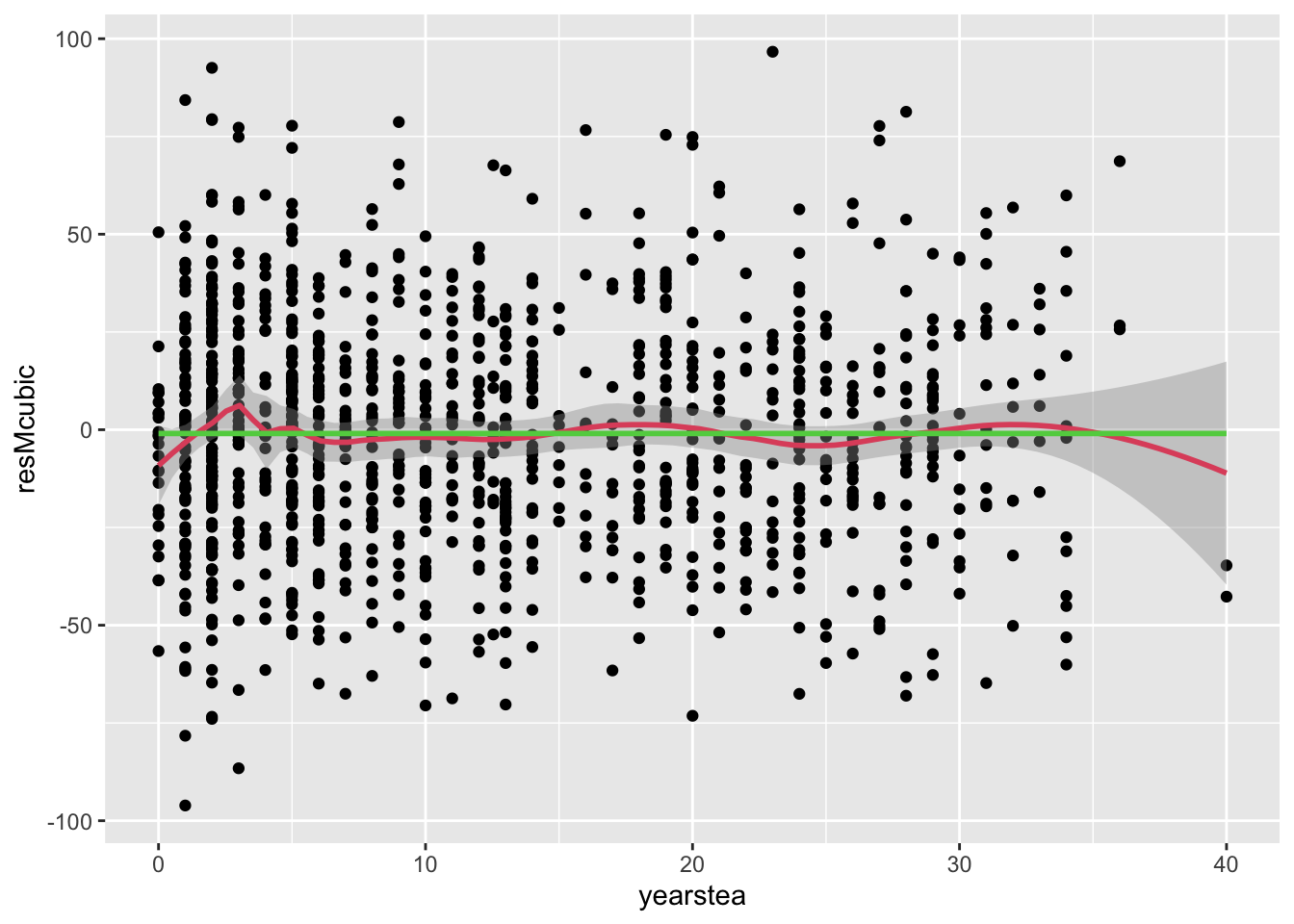

(cont.)
1. (cont.)
1. We have to consider that the early “phase” prior to ten years of teaching may be important. 1. There are a lot of observations in that range, so what we see may be “real” 2. What happens AFTER 7 or so years seems distinctly different from what happens before…
We now look more closely at ‘new teachers’ and propose a two-phase model (again, we are digging a lot here – this discussion is to illustrate a non-linear model). Better to have a theoretical basis for a jump process.
1. The approach is fairly straightforward: assume that there are early and late career teachers, and model each separately.
  1. Imagine you had an indicator variable for early career (say first 7 years) and one for late career (after 7 years). Call these indicators PHASE1 and PHASE2, respectively.
  2. Then a model that allowed for different slopes in each phase would consist of a linear effect interacted with at least one phase indicator:
    \[ Y_{ijk} = {b_0} + {b_1}YEARSTE{A_{jk}} + {b_2}YEARSTEA_{jk}\times PHASE{2_{jk}} + {\zeta_k} + {\varepsilon_{ijk}} \]
(cont.)
1. However, in our residual analysis, there was very little indication of a ‘slope’ in the second phase. It seemed fairly flat.
2. A simplification to the above model would only allow a slope, or rise, in the first phase, followed by a flat 2^nd phase, as follows:
  \[ {Y_{ijk}} = {b_0} + {b_1}YEARSTE{A_{jk}} \times PHASE{1_{jk}} + {b_2}PHASE{2_{jk}} + {\zeta_k} + {\varepsilon_{ijk}} \] where PHASE1 and PHASE2 are the phase indicators.
  1. The code and model fit along with Wald test.
    1. The LRT is conducted on the full span of YEARSTEA (both phases), although a test of just the first phase slope is interesting as well.

Code

#*PHASE1 interaction is implicit in this variable construction:
#*now look closely and make your own 'bump' at time pt 8
#R has a way with a true/false factor:
dat$yt_early <- (dat$yearstea<8)*dat$yearstea
dat$yt_late <- dat$yearstea>7
#we'll add the square term in the R formula
#*linear version
fit.MearlyLin <-lmer(mathgain~yt_early+yt_late+(1|schoolid),data=dat,REML=F)
print(summary(fit.MearlyLin))

## Linear mixed model fit by maximum likelihood . t-tests use Satterthwaite's method [lmerModLmerTest
## ]
## Formula: mathgain ~ yt_early + yt_late + (1 | schoolid)
##    Data: dat
## 
##      AIC      BIC   logLik deviance df.resid 
##  11787.3  11812.7  -5888.7  11777.3     1185 
## 
## Scaled residuals: 
##     Min      1Q  Median      3Q     Max 
## -4.8304 -0.5927 -0.0234  0.5415  5.6388 
## 
## Random effects:
##  Groups   Name        Variance Std.Dev.
##  schoolid (Intercept)  109.2   10.45   
##  Residual             1091.2   33.03   
## Number of obs: 1190, groups:  schoolid, 107
## 
## Fixed effects:
##             Estimate Std. Error       df t value Pr(>|t|)    
## (Intercept)  53.3445     3.3841 538.5144  15.763   <2e-16 ***
## yt_early      0.9968     0.8073 953.5928   1.235    0.217    
## yt_lateTRUE   4.8700     3.5992 797.2556   1.353    0.176    
## ---
## Signif. codes:  0 '***' 0.001 '**' 0.01 '*' 0.05 '.' 0.1 ' ' 1
## 
## Correlation of Fixed Effects:
##             (Intr) yt_rly
## yt_early    -0.815       
## yt_lateTRUE -0.880  0.776

Code

#test  yt_early yt_late
anova(fit.Mconst,fit.MearlyLin,refit=F)

## Data: dat
## Models:
## fit.Mconst: mathgain ~ 1 + (1 | schoolid)
## fit.MearlyLin: mathgain ~ yt_early + yt_late + (1 | schoolid)
##               npar   AIC   BIC  logLik deviance  Chisq Df Pr(>Chisq)
## fit.Mconst       3 11785 11800 -5889.6    11779                     
## fit.MearlyLin    5 11787 11813 -5888.7    11777 1.9093  2     0.3849

(cont.)
1. (cont.)
  1. (cont.)
    1. Let’s not get too discouraged by this null finding. Whatever is going on in phase one could be more complex.
  2. Let’s examine residuals, as we always do for completeness.

Code

#predict resMearlyLin, residual
resMearlyLin <- residuals(fit.MearlyLin)
dat$resMearlyLin <- resMearlyLin
#twoway (scatter resMearlyLin yearstea if abs(resMearlyLin)<100, jitter(1) msize(small) ) (lowess resMearlyLin yearstea, bwidth(.2) lwidth(1))
#graph copy gMearlyLin, replace
bool <- abs(dat$resMearlyLin) < 100 #selection crit

ggplot(data=dat[bool,],aes(y=resMearlyLin,x=yearstea))+
  geom_point()+
  stat_smooth(method="loess",span=.3,col=2)+
  geom_smooth(col=3,se=F)

## `geom_smooth()` using formula = 'y ~ x'
## `geom_smooth()` using method = 'gam' and formula = 'y ~ s(x, bs = "cs")'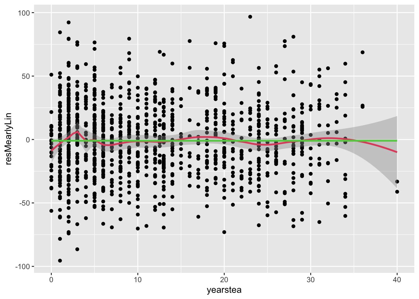

(cont.)

(cont.)
1. Comment: it seems the early phase itself is non-linear, so let’s model it that way.
A quadratic functional form for the mean in phase one could be modeled:

\[ {Y_{ijk}} = {b_0} + ({b_{11}}YEARSTE{A_{jk}} + {b_{12}}YEARSTEA_{jk}^2) \times PHASE{1_{jk}} + {b_2}PHASE{2_{jk}} + {\zeta_k} + {\varepsilon_{ijk}} \] 4. (cont.)
d. (cont.) i. The code to generate the quadratic, phase one term and fit the new model, along with LRT:

Code

#*quadratic version
fit.MearlyQuad <-lmer(mathgain~yt_early+I(yt_early^2)+yt_late+(1|schoolid),data=dat,REML=F)
print(summary(fit.MearlyQuad))

## Linear mixed model fit by maximum likelihood . t-tests use Satterthwaite's method [lmerModLmerTest
## ]
## Formula: mathgain ~ yt_early + I(yt_early^2) + yt_late + (1 | schoolid)
##    Data: dat
## 
##      AIC      BIC   logLik deviance df.resid 
##  11782.0  11812.5  -5885.0  11770.0     1184 
## 
## Scaled residuals: 
##     Min      1Q  Median      3Q     Max 
## -4.8485 -0.6116 -0.0249  0.5591  5.6736 
## 
## Random effects:
##  Groups   Name        Variance Std.Dev.
##  schoolid (Intercept)  102     10.10   
##  Residual             1088     32.98   
## Number of obs: 1190, groups:  schoolid, 107
## 
## Fixed effects:
##                Estimate Std. Error        df t value Pr(>|t|)    
## (Intercept)     43.2472     5.0186  882.2713   8.617  < 2e-16 ***
## yt_early         9.5455     3.2467 1067.7778   2.940  0.00335 ** 
## I(yt_early^2)   -1.1946     0.4389 1050.2186  -2.722  0.00660 ** 
## yt_lateTRUE     14.9370     5.1594 1006.4627   2.895  0.00387 ** 
## ---
## Signif. codes:  0 '***' 0.001 '**' 0.01 '*' 0.05 '.' 0.1 ' ' 1
## 
## Correlation of Fixed Effects:
##             (Intr) yt_rly I(_^2)
## yt_early    -0.856              
## I(yt_rly^2)  0.743 -0.969       
## yt_lateTRUE -0.945  0.831 -0.721

Code

#test  yt_early yt_early_sq yt_late
anova(fit.Mconst,fit.MearlyQuad,refit=F)

## Data: dat
## Models:
## fit.Mconst: mathgain ~ 1 + (1 | schoolid)
## fit.MearlyQuad: mathgain ~ yt_early + I(yt_early^2) + yt_late + (1 | schoolid)
##                npar   AIC   BIC  logLik deviance  Chisq Df Pr(>Chisq)  
## fit.Mconst        3 11785 11800 -5889.6    11779                       
## fit.MearlyQuad    6 11782 11812 -5885.0    11770 9.2453  3     0.0262 *
## ---
## Signif. codes:  0 '***' 0.001 '**' 0.01 '*' 0.05 '.' 0.1 ' ' 1

(cont.)
1. (cont.)
  1. (cont.)
    1. Finally, something is significant! (unfortunately, we should not trust this p-value, due to so much model exploration)
    2. Below, we test the first phase separately (using a Wald test), since the second phase has a large coefficient (approx. 15), and this could be driving the test results (we see that it is not). Followed by residuals.

Code

#test  yt_early yt_early_sq
#require(aod) # for this version of a Wald test
#print(wald.test(b=fixef(fit.MearlyQuad),Sigma=summary(fit.MearlyQuad)$vcov,Terms=2:3))
resMearlyQuad <- residuals(fit.MearlyQuad)
dat$resMearlyQuad <- resMearlyQuad
bool <- abs(dat$resMearlyQuad) < 100 #selection crit

ggplot(data=dat[bool,],aes(y=resMearlyQuad,x=yearstea))+
  geom_point()+
  stat_smooth(method="loess",span=.3,col=2)+
  geom_smooth(col=3,se=F)

## `geom_smooth()` using formula = 'y ~ x'
## `geom_smooth()` using method = 'gam' and formula = 'y ~ s(x, bs = "cs")'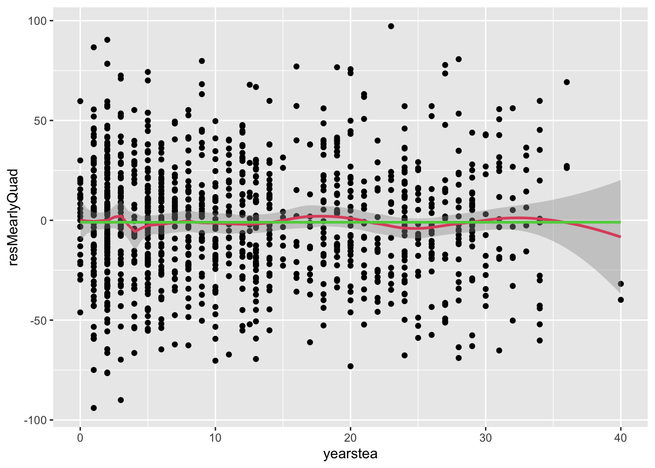

(cont.)
1. (cont.)
  1. (cont.)
    1. Comment: we see an improvement in our predictions in the early phase. For now, let us call this success… with the caveat that we ‘dug’ or ‘snooped’ too much if this were a real problem.

4.3 Information Criteria

The models we’ve explored have not all been nested. We need some additional model selection tools to compare some of these non-nested models (polynomial vs. non-parametric, e.g.). We will use of Information Criteria (IC) in model selection in this situation.
1. An information criterion is a measurement, based on the log-likelihood, used to assess goodness of fit (the better fitting model is selected).
  1. As long as the estimation methods are the same (REML vs. FML, e.g.) and the observations included in the estimation are identical, this approach allows us to compare non-nested models (non-nested with respect to parameters).
2. The idea is to compare log-likelihoods, but a simple comparison won’t work, because the likelihood should always improve, or at least won’t get worse with the addition of new predictors.
  1. The idea is to ‘penalize’ the log-likelihood for the number of parameters.
  2. Given two models with the same log-likelihoods and different numbers of parameters, an IC will favor the model with fewer parameters, satisfying the goal of ‘parsimony’ (the simpler model is preferred).
3. We will describe the AIC (Akaike’s IC) and BIC (Bayesian, or Schwarz’s IC), but these are only two possibilities – there are many different choices – but these are the most common in use right now.¹¹
  1. The formula used in the AIC calculation is \(AIC = - 2\ln (L) + 2p\), where ln(L) is the loglikelihood of the model evaluated at the MLEs for the parameters and p is the number of parameters in the model (including the constant, all fixed effects and all random effects variances/covariances).
    1. We choose the model with the smaller AIC.
  2. The formula used in the BIC calculation is \(BIC = - 2\ln (L) + p\ln (N)\), where ln(L) is the loglikelihood of the model evaluated at the MLEs for the parameters, p is the number of parameters in the model and N is the number of observations.
    1. We choose the model with the smaller BIC.
    2. There is some debate over whether N should be the number of observations or the number of subjects, when there are repeated measures for subjects. STATA uses the number of observations, and this yields a larger penalty term; R seems to do the same.
    3. A difference of 2 BIC points is understood as weakly significantly different. Larger differences are moderate and stronger evidence of one model’s superiority to another.
  3. There is a concern that the expression for ln(L) may vary with software implementation under REML estimation. 1. The number of parameters in the model is also less clear in this instance, because REML estimation is conditional on the fixed effects. 2. Given the above controversy, when comparing models with different fixed effects, FIML not REML estimation is slightly preferred. In STATA, implementation is correct, so the estimation technique is not crucial. Since it may be an issue in other packages, we make the point here, and we used FIML throughout the following notes to avoid the issue. 3. In R, there are several ways to reveal the ICs.
    - On a model fit, one can call the function: BIC
    - To compare several models, store the estimates from each, and then call anova on the fit objects, listing them in increasing order of complexity.
4. Below are the results from a set of models, each with a different form for YEARSTEA, from excluding it (Mconst) to linear (Mlin) to multiphase (MearlyLin, MearlyQuad). These are non-nested (do not share common parameters). We list the IC comparisons for our alternative, non-linear models for YEARSTEA. We had stored the models as we fit each one, so they are fairly easily recalled and summarized:

Code

#*Info Crit:
anova(fit.Mconst,fit.Mlin,fit.Mcubic,fit.MearlyLin,fit.MearlyQuad,refit=F)

## Data: dat
## Models:
## fit.Mconst: mathgain ~ 1 + (1 | schoolid)
## fit.Mlin: mathgain ~ yearstea + (1 | schoolid)
## fit.MearlyLin: mathgain ~ yt_early + yt_late + (1 | schoolid)
## fit.Mcubic: mathgain ~ yearstea + I(yearstea^2) + I(yearstea^3) + (1 | schoolid)
## fit.MearlyQuad: mathgain ~ yt_early + I(yt_early^2) + yt_late + (1 | schoolid)
##                npar   AIC   BIC  logLik deviance  Chisq Df Pr(>Chisq)
## fit.Mconst        3 11785 11800 -5889.6    11779                     
## fit.Mlin          4 11787 11807 -5889.3    11779 0.6833  1     0.4084
## fit.MearlyLin     5 11787 11813 -5888.7    11777 1.2260  1     0.2682
## fit.Mcubic        6 11789 11820 -5888.7    11777 0.0218  1     0.8826
## fit.MearlyQuad    6 11782 11812 -5885.0    11770 7.3142  0

(cont.)
1. (cont.)
  1. If one were only using AIC, one might conclude that the two-phase model with quadratic growth in the early phase was best
  2. BIC penalizes more heavily for too many parameters, and so it actually prefers a model with no YEARSTEA terms of any kind.
  3. There is no way to resolve this difference. Each IC serves a different function. Many researchers prefer the use of AIC (based on more ‘classical’ assumptions) to BIC (based on Bayesian approach). 1. I tend to use BIC when exploring a limited class of models (not looking for a ‘true’ model). 2. Some statisticians would argue that BIC is useful when your goal is description (simpler stories are better) and that AIC is useful when your goal is prediction (more complex models may do a better job).

4.4 Appendix

4.1.e. Matrix form (optional):

\[ Y_{ijk} = {b_0} + {\zeta_k} + {\eta_{jk}} + {\varepsilon_{ijk}},\mbox{ with }\zeta_k\sim N(0,\sigma_\zeta^2),\ \eta_{jk}\sim N(0,\sigma_\eta^2)\ \varepsilon_{ijk} \sim N(0,\sigma_\varepsilon^2), \mbox{indep.} \] This translates, in matrix form (assuming complete balanced design for simplicity, and \(n_I\) students (each) in \(n_J\) classrooms in \(n_K\) schools, to: \[ Y = X\beta + Z\delta + \varepsilon \mbox{ with }\delta = \begin{vmatrix} \zeta&0 \\ 0&\eta \\ \end{vmatrix},\\ \zeta\sim N(0_{n_K},\sigma_\zeta^2I_{n_K}),\ \eta\sim N(0_{n_Jn_K},\sigma_\eta^2I_{n_Jn_K})), \ \varepsilon \sim N(0_{n_In_Jn_K},\sigma_\varepsilon^2I_{n_In_Jn_K})), \mbox{indep. of ea. other} \] Note that \(I_n\) is an \(n \times n\) identity matrix and \(0_n\) is a zero vector of length \(n\). The design matrix \(X\) is simply a column of ones in our example, as it’s just the intercept. The design matrix \(Z\) is more complex, but it identifies which component of the \(\zeta\) or \(\eta\) corresponding to the school or classroom to ‘pick.’
\[ \mbox{Let }G=\begin{vmatrix} \sigma_\zeta^2I_{n_K}&0\\ 0&\sigma_\eta^2I_{n_Jn_K}\\ \end{vmatrix} \] \[ \mbox{And let }\Sigma = ZGZ' + \sigma_\varepsilon^2I_{n_In_Jn_K}, \mbox{ and } u = \begin{vmatrix} \zeta\\ \eta\\ \end{vmatrix} \] \[ \mbox{Then }\hat{u}= \hat{G}\hat{Z}'\hat{\Sigma}^{-1}(Y-X\hat{\beta}) \] is the expression for the BLUPs of this model, where the ‘hat’ signifies estimation from a sample. You should recognize \((Y-X\hat{\beta})\) as the set of ‘fixed effects residuals.’

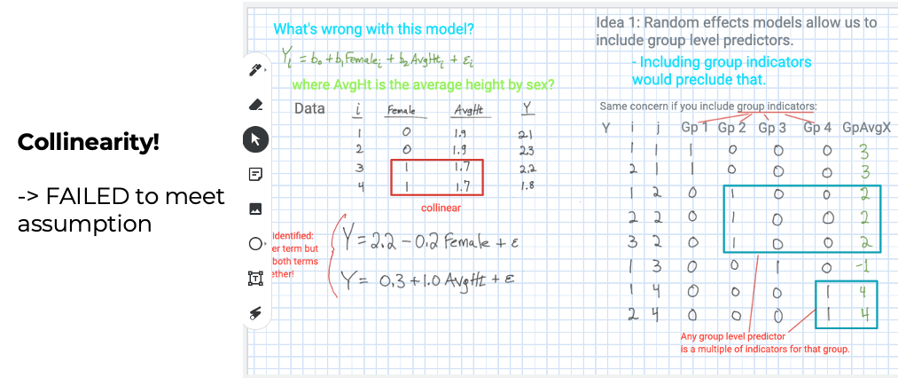
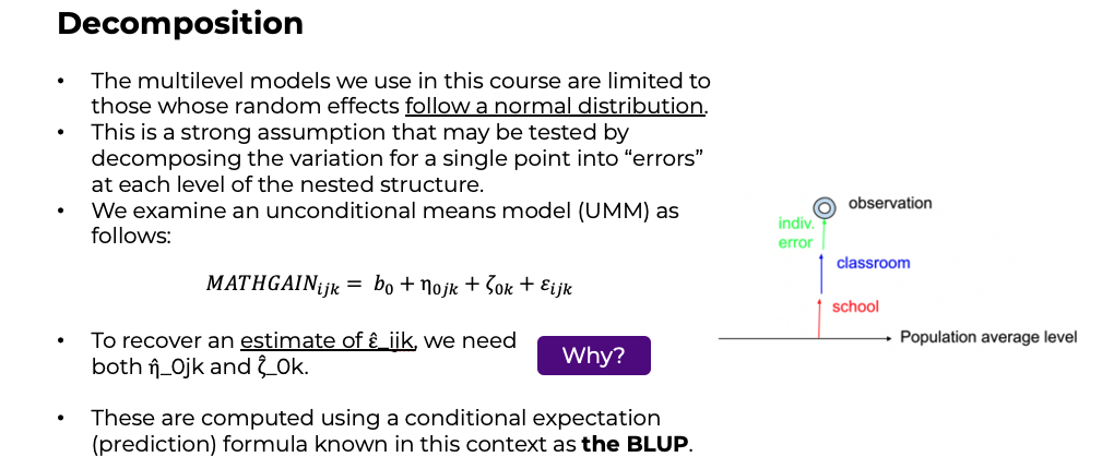
\[ \\ \] [Additional support material on chapter 4 concepts]

Images from the Jamboard slides “Jamboard: MLM Module 4”
Slides are directly sourced from the slides “W4_slides”

Model assumption is important

Decomposition

Visualize the BLUPs

4.4.0.0.0.0.0.0.0.0.0.0.0.0.0.0.0.0.0.0.0.0.0.0.0.0.0.0.0.0.0.0.0.0.0.0.0.0.0.0.0.0.0.0.0.0.0.0.0.0.0.0.0.0.0.0.0.0.0.0.0.0.0.0.0.0.0.0.0.0.0.0.0.0.0.0.0.0.0.0.0.0.0.0.0.0.0.0.0.0.0.0.0.0.0.0.0.1

4.5 Coding

4.5.0.0.0.0.0.0.0.0.0.0.0.0.0.0.0.0.0.0.0.0.0.0.0.0.0.0.0.0.0.0.0.0.0.0.0.0.0.0.0.0.0.0.0.0.0.0.0.0.0.0.0.0.0.0.0.0.0.0.0.0.0.0.0.0.0.0.0.0.0.0.0.0.0.0.0.0.0.0.0.0.0.0.0.0.0.0.0.0.0.0.0.0.0.0.0.1

ranef()
residuals()

ranef() is a function to extract the random effects from a fitted model from the lme4 library. It has arguments as follows:
- object: an object of fitted models with random effects

Code

# extract the random effects
lme4::ranef(fit2)

## $`classid:schoolid`
##           (Intercept)
## 1:61     -1.324428250
## 2:34      2.245432176
## 3:56     -8.759950590
## 4:67      9.425092900
## 5:15     10.309267405
## 6:21     -5.699024642
## 7:17     -1.117503647
## 8:76     -7.531898940
## 9:40    -13.300777367
## 10:17     6.843162206
## 11:3      3.869435956
## 12:58    -1.927220451
## 13:78    -4.198141517
## 14:53     8.237489677
## 15:91    -1.703917732
## 16:38     0.727065313
## 17:9     -2.383605526
## 18:41     0.334968488
## 19:46     3.770488684
## 20:12    -1.246382332
## 21:87    -1.158895586
## 22:62    -2.638123658
## 23:79    -0.815054748
## 24:55    -3.131548033
## 25:50    -4.232889584
## 26:33     7.685564435
## 27:77    -1.602190079
## 28:76     2.800365782
## 29:72     1.503284375
## 30:20    -1.446646225
## 31:18     7.393331925
## 32:33    -7.783724121
## 33:105    0.968216684
## 34:59    -4.282804584
## 35:55     1.299341747
## 36:57     2.416509330
## 37:103    0.096024647
## 38:64     3.506238652
## 39:75    -0.234879389
## 40:57     7.212182379
## 41:14    -5.259897835
## 42:75     8.028252758
## 43:23    -1.756184982
## 44:102   -6.990128045
## 45:91    -9.425758410
## 46:62     1.202374713
## 47:23     4.943799485
## 48:4      3.770020516
## 49:12     0.103204113
## 50:41    -1.307146586
## 51:31    -2.713228021
## 52:90    -7.464038826
## 53:77     2.157924125
## 54:42    -1.091523611
## 55:24    -8.911586268
## 56:35    -5.814033357
## 57:68    -4.633141651
## 58:9     -0.905044510
## 59:51    -0.212041489
## 60:104    0.087070810
## 61:47    -1.890081419
## 62:106   -6.883393778
## 63:36    -0.942172855
## 64:13    -0.269972304
## 65:86    -2.686421250
## 66:85    -6.479592754
## 67:88    -5.078802092
## 68:101   -6.282242525
## 69:46    -4.084147150
## 70:42    -0.696938640
## 71:46     3.608717955
## 72:87    -1.682539087
## 73:67     3.488109935
## 74:100   -4.247190458
## 75:97     2.396112375
## 76:84     2.110868544
## 77:24    -5.982663091
## 78:26     4.477552395
## 79:39    -8.869332549
## 80:71    -1.609833188
## 81:12     3.026981612
## 82:47     9.671273498
## 83:70     6.599894805
## 84:85     0.791640227
## 85:15     6.509301051
## 86:11     1.766389170
## 87:17    -0.853492951
## 88:33    -5.977387990
## 89:7     -0.607948136
## 90:69     4.408462041
## 91:66     1.711240997
## 92:15     2.564953669
## 93:24     4.753771862
## 94:20     1.395349441
## 95:65    -5.770924096
## 96:107   -3.746560335
## 97:25    -2.745101255
## 98:19    -1.067975004
## 99:100   -0.023019329
## 100:33   -1.711647331
## 101:20    2.314193604
## 102:26   -0.695322653
## 103:37   -7.769202626
## 104:27    0.598408638
## 105:49   10.798399523
## 106:87   -4.717453721
## 107:7    -1.589631517
## 108:59    0.748415885
## 109:96   -1.276946772
## 110:19   -1.429070448
## 111:78   -1.179593660
## 112:79   -0.123206295
## 113:11   -0.712225251
## 114:28   -6.377868954
## 115:29    0.265716559
## 116:81    4.446497382
## 117:55   -0.526850672
## 118:28    1.482718073
## 119:15   -2.275242417
## 120:71    4.967043189
## 121:60    8.956619770
## 122:35   -6.428239927
## 123:93   -2.110686877
## 124:61    0.011485797
## 125:37    5.818469668
## 126:93   -8.712806483
## 127:50    0.404222502
## 128:65    4.059415509
## 129:104   9.964962113
## 130:21    2.113453536
## 131:11   -0.594107931
## 132:86   -5.655753724
## 133:46   -1.315344284
## 134:94    8.409281750
## 135:100   5.481081988
## 136:76   -1.636172901
## 137:3     5.563998670
## 138:101   5.985663782
## 139:26   -4.204429344
## 140:95   -2.036762724
## 141:14   -4.153355803
## 142:41    5.794346844
## 143:84    7.179423151
## 144:95    4.806396020
## 145:3     8.101953467
## 146:70    4.829747971
## 147:8     7.746431575
## 148:72   -3.960251903
## 149:53   -2.484372952
## 150:24    3.169707689
## 151:91    3.904835282
## 152:70    4.710671349
## 153:48   -2.402018016
## 154:75    0.007776705
## 155:47   -1.051480116
## 156:31   -0.635391787
## 157:85    1.808944547
## 158:21    2.924973884
## 159:22   -4.100503083
## 160:1     1.638385370
## 161:84    3.503318236
## 162:7     4.415040388
## 163:23    1.159646182
## 164:82   -0.241084960
## 165:83    3.628520547
## 166:13   -3.823534963
## 167:14    2.160442854
## 168:56    5.252008993
## 169:82    3.566263859
## 170:19    1.798648245
## 171:57    0.656438027
## 172:11  -11.326890503
## 173:92   -0.802665018
## 174:81   -0.495018652
## 175:30   -5.684331960
## 176:44    3.407528277
## 177:17    4.482828643
## 178:10    3.442918977
## 179:4   -12.045874449
## 180:36    5.931321249
## 181:75    1.192278672
## 182:93    2.995843982
## 183:78   -6.792031900
## 184:82   -3.886164597
## 185:96   -3.659650506
## 186:85   -6.846269737
## 187:87    2.097885721
## 188:34   -4.501687243
## 189:77   -0.275026027
## 190:27    2.181312271
## 191:32    3.861594850
## 192:61   -4.184925436
## 193:103   1.794222612
## 194:93   -2.199251119
## 195:11    1.622891633
## 196:85    8.904069037
## 197:2    -1.694597106
## 198:39   -5.654246674
## 199:92   -2.196722504
## 200:105   0.755354581
## 201:11   -5.263407273
## 202:28  -10.435755745
## 203:28   11.137653693
## 204:32   -3.901912918
## 205:99    0.303230576
## 206:16    7.340627601
## 207:42   -2.048295429
## 208:10   -0.199758985
## 209:71    3.280117671
## 210:37   -0.285951639
## 211:2     2.513287831
## 212:49   -1.455157767
## 213:73   -1.789358023
## 214:99   -2.709810600
## 215:101  -4.983871258
## 216:17   -1.326259631
## 217:1    -0.432890686
## 218:66   -1.392083408
## 219:44   -1.117933222
## 220:43   -1.543012866
## 221:98   -1.210309581
## 222:80    7.281657838
## 223:29   -5.234459724
## 224:94   -4.183380294
## 225:82   -0.061534653
## 226:99    0.599837004
## 227:43    1.045318806
## 228:3    -0.023718744
## 229:33    9.096507820
## 230:27   -7.096561976
## 231:91    2.020601630
## 232:74    0.068253684
## 233:11    0.072820270
## 234:31    9.428198374
## 235:83   -4.255034577
## 236:99    4.158793052
## 237:96    0.018277210
## 238:90    6.455975613
## 239:107   0.287168386
## 240:46   -3.560319580
## 241:102   5.457818125
## 242:60   -0.874348298
## 243:72   -0.687995126
## 244:68   12.858495085
## 245:67   -2.199160815
## 246:44    5.844315238
## 247:103  14.089256338
## 248:92    4.964166696
## 249:37   -1.373478156
## 250:57   -2.594928547
## 251:12    0.474765395
## 252:32   -1.632941455
## 253:79    3.286935212
## 254:6     5.716593494
## 255:52   -0.934923446
## 256:16    3.692195805
## 257:40    4.108596510
## 258:31  -11.875808102
## 259:54   -6.765728529
## 260:15   -7.600134884
## 261:70   -0.042805750
## 262:27    4.241303244
## 263:68   -2.144697617
## 264:71   -6.972552012
## 265:8     0.320808805
## 266:99   -5.725396485
## 267:61   -1.617014891
## 268:44   -0.981004158
## 269:66    0.549165345
## 270:52   -5.735848906
## 271:68    0.698937758
## 272:57   -2.423686755
## 273:101   8.328929263
## 274:39    0.224213425
## 275:86   -0.492310543
## 276:73   -0.928795964
## 277:76   -6.137614609
## 278:10    5.133189001
## 279:8   -12.969187875
## 280:7    -1.857701596
## 281:100  -0.142467845
## 282:94    3.711990908
## 283:9    -4.575552439
## 284:65    0.746796612
## 285:11    4.301552910
## 286:6     0.429363741
## 287:76    2.735275074
## 288:39   -1.031031964
## 289:50   -2.863807106
## 290:69   -2.076311188
## 291:6     5.037221780
## 292:89   -1.755989475
## 293:11    4.686280956
## 294:64    0.541341759
## 295:74    0.125133691
## 296:42    4.467151917
## 297:25   -7.442824641
## 298:68    6.611049290
## 299:5     0.780900164
## 300:45    2.380272097
## 301:54   -1.743893797
## 302:12   -6.039397885
## 303:10    2.237027976
## 304:71   -3.125677486
## 305:77   -1.634592899
## 306:94    6.947209573
## 307:2     2.443665346
## 308:80   -1.295290892
## 309:38   -5.092460890
## 310:63   -0.463570406
## 311:70   -1.939050171
## 312:88   -1.363225535
## 
## $schoolid
##      (Intercept)
## 1     0.94162990
## 2     2.54827506
## 3    13.67862651
## 4    -6.46439313
## 5     0.60997278
## 6     8.73534818
## 7     0.28101324
## 8    -3.82898441
## 9    -6.14284602
## 10    8.29026729
## 11   -4.25449562
## 12   -2.87515059
## 13   -3.19749967
## 14   -5.66527884
## 15    7.42695395
## 16    8.61790316
## 17    6.27136454
## 18    5.77504200
## 19   -0.54552849
## 20    1.76758251
## 21   -0.51600236
## 22   -3.20296421
## 23    3.39571026
## 24   -5.44497242
## 25   -7.95794110
## 26   -0.32978642
## 27   -0.05900372
## 28   -3.27541250
## 29   -3.88115951
## 30   -4.44011660
## 31   -4.52752147
## 32   -1.30700801
## 33    1.02272380
## 34   -1.76239454
## 35   -9.56262253
## 36    3.89709834
## 37   -2.81995205
## 38   -3.40987569
## 39  -11.97480269
## 40   -7.18014978
## 41    3.76666804
## 42    0.49241035
## 43   -0.38875626
## 44    5.58724183
## 45    1.85926609
## 46   -1.23463369
## 47    5.25667854
## 48   -1.87625215
## 49    7.29814570
## 50   -5.22759156
## 51   -0.16562877
## 52   -5.21063993
## 53    4.49384541
## 54   -6.64699311
## 55   -1.84269463
## 56   -2.74010558
## 57    4.11375309
## 58   -1.50538068
## 59   -2.76076381
## 60    6.31318298
## 61   -5.55754122
## 62   -1.12148495
## 63   -0.36210177
## 64    3.16162552
## 65   -0.75355093
## 66    0.67826001
## 67    8.36889826
## 68   10.45963116
## 69    1.82167787
## 70   11.05938319
## 71   -2.70336211
## 72   -2.45657731
## 73   -2.12319068
## 74    0.15105777
## 75    7.02490153
## 76   -7.63152855
## 77   -1.05753970
## 78   -9.50598685
## 79    1.83458448
## 80    4.67604064
## 81    3.08655906
## 82   -0.48625994
## 83   -0.48937947
## 84    9.99327982
## 85   -1.42257330
## 86   -6.90074860
## 87   -4.26567076
## 88   -5.03196401
## 89   -1.37162961
## 90   -0.78741323
## 91   -4.06510900
## 92    1.53471836
## 93   -7.83216175
## 94   11.62697547
## 95    2.16340194
## 96   -3.84177327
## 97    1.87163917
## 98   -0.94539089
## 99   -2.63497130
## 100   0.83454660
## 101   2.38121269
## 102  -1.19691017
## 103  12.48182895
## 104   7.85179307
## 105   1.34630726
## 106  -5.37672170
## 107  -2.70218273
## 
## with conditional variances for "classid:schoolid" "schoolid"

residuals() is a function to extracts model residuals from stats library. resid() is an abbreviated form of the function. It has an argument as follows:
- object: an object for which the extraction of model residuals

Code

residuals(fit.M3)[1:5] # print out first 5 residuals

##          1          2          3          4          5 
## -0.3398926  0.4601074  0.2101074  0.3001074  0.1601074

4.6 Quiz

4.6.1 Self-Assessment

Use “W4 Activity Form” to submit your answers.
1. Compute the following questions using multi-level equations based on the chapter 4 content as follows:
- Given level 1: \(Y_{ij} = \beta_{0k} + \beta_{1k} + \epsilon_{ik}\) and
- level 2: \(\beta_{0k} = b_0 + \zeta_{0k}; \beta_{1k}=b_1 + \zeta_{1k}\) with \(\varepsilon_{ijk}\sim N(0,\sigma_\varepsilon^2)\), \(\zeta_{0k}\sim N(0,\sigma_{\zeta_0}^2)\), \(\zeta_{1k}\sim N(0,\sigma_{\zeta_1}^2)\), independently.
- 1-A: \(E(Y_{ik} | X_{ik})\)
- 1-B: \(E(\zeta_{0k})\)
- 1-C: \(E(\zeta_{1k})\)
- 1-D: \(E(\beta_{0k})\)
- 1-E: \(E(\beta_{1k})\)
- 1-F: Does \(E(Y_{ik}) = E(Y_{ik} | \zeta_{0k}, \zeta_{1k}, X_{ik})\)?
- 1-G: Does \(E \zeta_{0k} | Y_{ik},X_{ik}, b_0, b_1, \sigma_\varepsilon^2 , \sigma_{\zeta_0}^2, \sigma_{\zeta_1}^2 ) = E(\zeta_{0k})\)?
1. In the doubly nested model \(MATHGAIN_{ijk} = b_0 + eta_{jk} + \zeta_k + \epsilon_{ijk}\), the BLUPs for classrooms and schools (assuming a single student in a single classroom) are given by:
\[\hat\zeta_k | \hat e_k, \hat\sigma_\eta^2, \hat\sigma_\zeta^2, \hat\sigma_\epsilon^2 = \frac{\hat\sigma_\zeta^2}{\hat\sigma_\eta^2 + \hat\sigma_\zeta^2 + \hat\sigma_\epsilon^2}\hat e_k\]

\[\hat\eta_k | \hat e_k, \hat\sigma_\eta^2, \hat\sigma_\zeta^2, \hat\sigma_\epsilon^2 = \frac{\hat\sigma_\eta^2}{\hat\sigma_\eta^2 + \hat\sigma_\zeta^2 + \hat\sigma_\epsilon^2}\hat e_k\]

Using this decomposition and assuming all variance components are equal to one; we draw a picture with the single observation’s residual divided into a portion attributable to schools, classrooms and individuals.
- 2-A: Does this single observation contain any information about the three variance components? HINT: how many observations do you need to estimate a mean? How many for a variance?
- 2-B: Give an explicit numeric expression for these three “residuals” (you have enough information):
- 2-C: True or False: One can compute the Level 1 residual without knowing the Level 2 or 3 residuals? Why or why not?
- 2-D: True or False: Level 2 always has “at least as many” errors as does Level 3. Why or why not?

4.6.2 Lab Quiz

Review the material in the Rshiny app “Week4: Handout4 Activity” and then answer these questions on the google form “W4 Activity Form”

4.6.3 Homework

Homework is presented as the last section of the Rshiny app “Week4: Handout4 Activity”.
Follow instructions there (fill out this form “W4 Activity Form” ) and hand in your code on Brightspace

We are of course assuming that treatment did not change the sex ratios.↩︎
Independence between slope and intercept within classroom is a strong assumption that can be changed to allow correlation.↩︎