2.1 Model Specification and Related Theory
2.1.1 Discrete-geographic model
The process of geographic dispersal over the tree, \(\Psi\), is described as a continuous-time Markov chain (CTMC). For a biogeographic history with \(k\) discrete-geographic areas, this stochastic process is fully specified by a \({k \times k}\) instantaneous-rate matrix, \(\mathbf{Q}\), where an element of the matrix, \(q_{ij}\), specifies the instantaneous rate of change between state \(i\) and state \(j\), i.e., the instantaneous rate of dispersal from area \(i\) to area \(j\). By convention, we rescale the \(\mathbf{Q}\) matrix such that the expected (average) number of dispersal events in one time unit is equal to the parameter \(\mu\): this is the average rate of dispersal among all \(k\) discrete geographic areas.
BSSVS
For most inference problems, the number of discrete geographic areas, \(k\), is large, such that the discrete-geographic model includes many parameters, while the data are limited to a single observation (the geographic area occupied by each tip in the tree). Accordingly, inference under these discrete-geographic models raises concerns about our ability to estimate each parameter in the matrix. (For details, see Inherent Prior Sensitivity of Biogeographic Inference.) This concern motivated Lemey and colleagues (Lemey et al. 2009) to develop an approach to reduce the complexity of the discrete-geographic model called Bayesian stochastic search variable selection (BSSVS).
This approach involves by specifying each element, \(q_{ij}\), of the instantaneous-rate matrix, \(\mathbf{Q}\), as: \[\begin{align*} q_{ij}= r_{ij}\delta_{ij}, \end{align*}\] where \(r_{ij}\) is the relative rate of dispersal between areas \(i\) and \(j\), and \(\delta_{ij}\) is an indicator variable that takes one of two states (0 or 1). When \({\delta_{ij}= 1}\), the instantaneous dispersal rate for the corresponding element, \(q_{ij}\), is simply \(q_{ij}= r_{ij}\).
Conversely, when \({\delta_{ij}= 0}\), the instantaneous dispersal rate for the corresponding element, \(q_{ij}\), is zero, effectively removing that parameter from the discrete-geographic model. The idea here is to exclude superfluous elements of the \(\mathbf{Q}\) matrix in order to reduce the number of parameters that must be inferred from the (inherently minimal amount of) data.
A given \(\mathbf{Q}\) matrix therefore entails a vector of \(\delta_{ij}\) (i.e., \(\boldsymbol{\delta}\)) and a vector of \(r_{ij}\) (i.e., \(\boldsymbol{r}\)). Each unique \(\boldsymbol{\delta}\) vector—a string of zeros and ones for each of the possible pairwise dispersal routes between the \(k\) geographic areas—corresponds to a unique discrete-geographic model.
By default, BEAST uses BSSVS to average over discrete-geographic models with different degrees of complexity. If BSSVS is not toggled in PrioriTree, the dispersal-route indicator vector, \(\boldsymbol{\delta}\), will be removed from the model and thus the rate matrix is simply \(\boldsymbol{r}\).
A/symmetry of the Instantaneous-Rate Matrix
Alternative discrete-geographic models may be specified based on the symmetry of the instantaneous-rate matrix. The discrete-geographic model described by Lemey et al. (2009) assumes that rate matrix, \(\mathbf{Q}\), is symmetric, where \({q_{ij}= q_{ji}}\) (i.e., \({r_{ij}= r_{ji}}\) and \({\delta_{ij}= \delta_{ji}}\)). Accordingly, this model assumes that the instantaneous rate of dispersal from area \(i\) to area \(j\) is equal to the dispersal rate from area \(j\) to area \(i\). For a dataset with \(k\) areas, the symmetric model has \(k \choose 2\) dispersal-route indicators and up to \(k \choose 2\) relative-rate parameters.
A subsequent extension (Edwards et al. 2011) allows the \(\mathbf{Q}\) matrix to be asymmetric, where \(q_{ij}\) and \(q_{ji}\) are not constrained to be equal. Accordingly, this model allows the rate of dispersal from area \(i\) to area \(j\) to be different from the rate of dispersal from area \(j\) to area \(i\). For a dataset with \(k\) areas, the asymmetric model has \({k \times (k - 1)}\) dispersal-route indicators and up to \({k \times (k - 1)}\) relative-rate parameters.
2.1.2 Inferring Biogeographic History
Empirical biogeographic studies often report summaries that are based on the conditional probability distribution of biogeographic histories over the tree. The distribution of histories depends on—i.e., is conditioned on—the instantaneous-rate matrix, \(\mathbf{Q}\), the discrete-geographic data, \(G\), and the phylogeny, \(\Psi\). Conceptually, for a given tree and rate matrix, we imagine simulating a geographic history over the tree from the root to its tips, where the rate matrix specifies the waiting times between dispersal events. We can construct the conditional distribution of biogeographic histories by simulating a large number of individual histories, and retaining only those histories that realize the observed geographic areas at the tips, \(G\). This conditional distribution contains all of the information required to compute two commonly reported summaries: the ancestral areas at internal nodes of the tree, and the number of dispersal events between geographic areas.
We can infer the total number of dispersal events among all \(k\) discrete geographic areas, and/or we can infer the number of dispersal events between each pair of geographic areas.
BEAST implements two algorithms for computing the number of dispersal events: the first option—referred to as fast stochastic mapping in PrioriTree—relies on analytical integration (Minin and Suchard 2008a, 2008b; O’Brien, Minin, and Suchard 2009).
As the name suggests, this is a more computationally efficient option for inferring biogeographic histories; however, this method only computes the expected (average) number of dispersal events on each branch, but does not allow us to infer all the details of the biogeographic history (such as the exact timing of dispersal events over the tree).
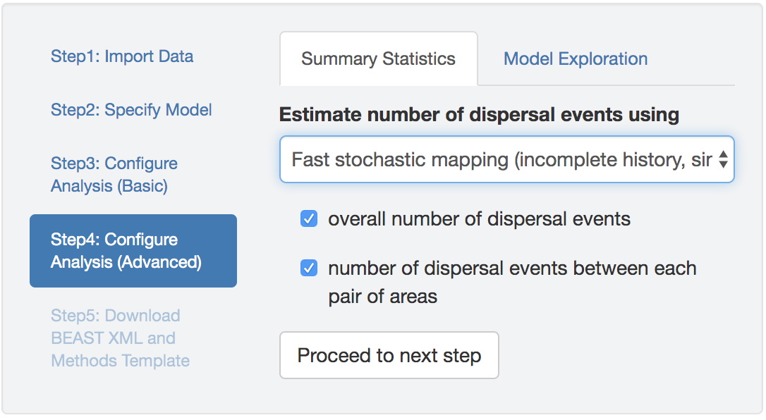
Figure 2.1: Options for inferring biogeographic history. You can specify either the integration-based or simulation-based methods for stochastic mapping of biogeographic histories, and for either method, you can choose to estimate the total and/or pairwise number of dispersal events.
The second option for inferring biogeographic histories—referred to as stochastic mapping in PrioriTree—relies on a simulation-based algorithm (Nielsen 2002; Rodrigue, Philippe, and Lartillot 2007; Hobolth and Stone 2009).
This method for mapping biogeographic histories is more computationally intensive, but also allows us to infer additional details (such as the exact timing of dispersal events over the tree).
When inferring biogeographic histories with either stochastic-mapping option, PrioriTree allows you to specify the type of dispersal events—i.e., the total number of dispersal events among all areas and/or the pairwise number of dispersal events between each pair of areas—in your BEAST analysis (Figure 2.1).
If you do not specify either type of dispersal event (total or pairwise number) and you are using the fast stochastic mapping algorithm (the first option), PrioriTree will not infer biogeographic histories (i.e., it will not write the part of XML script that instructs BEAST to perform computations for the expected number of dispersal events).
Conversely, if you do not specify either type of dispersal event (total or pairwise number) and you are using the stochastic mapping algorithm (the second option), PrioriTree will still write the part of the XML script that instructs BEAST to infer the full biogeographic history (i.e., the number of dispersal events will not be written to the parameter log file, but they can still be retrieved from the tree log file).
2.1.3 Accommodating Phylogenetic Uncertainty
The discrete-geographic model describes the process of dispersal over the phylogeny of our study group. Typically, the phylogeny and biogeographic history are inferred sequentially. Under this sequential-inference scenario, for example, we might first estimate the phylogeny for our study group from an alignment of sequence data using BEAST. The resulting phylogenetic estimate is then used to infer the biogeographic history of our study group.
PrioriTree requires that you provide an input file containing a previously inferred study tree.
If the input file includes a single tree (e.g., an MCC summary tree in a .tre file), the discrete-geographic inference will treat the phylogeny as a fixed variable (i.e., this effectively assumes that the phylogeny is ‘known’).
Alternatively, if the input file contains multiple trees (e.g., a posterior distribution of trees in a .trees file), the discrete-geographic inference will marginalize (i.e., `averaged’) over those trees to accommodate phylogenetic uncertainty.
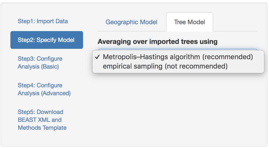
Figure 2.2: Specify the tree model.
BEAST provides two options for accommodating phylogenetic uncertainty in sequential analyses.
The first option—invoked with the argument MetropolisHastings = "true"—treats the posterior sample of trees as a prior distribution while inferring the joint posterior distribution of the biogeographic-model parameters.
Under this option, trees are proposed and accepted/rejected using the standard Metropolis–Hastings MCMC algorithm.
Specifically, the MCMC proposes a move to a new tree at a frequency specified by the corresponding proposal weight, and when a new tree is being proposed, it is randomly drawn from the posterior sample of trees, and the proposed tree is then accepted or rejected according to the computed acceptance probability.
Accordingly, sequential inference under this option is (theoretically) equivalent to performing joint inference of the phylogeny and biogeographic history (i.e., where the phylogeny and biogeographic history are simultaneously inferred from a single, combined dataset that includes both the sequence and geographic data).
The second option for accommodating phylogenetic uncertainty—invoked with the argument MetropolisHastings = "false"—averages over the posterior sample of trees using an ad hoc MCMC algorithm.
Similar to the previous option, the MCMC proposes a move to a new tree randomly drawn from the posterior sample of trees.
In contrast to the correct Metropolis–Hastings algorithm, however, proposed trees are always accepted (i.e., disregarding the acceptance probability of the proposed tree).
This procedure therefore ignores the fact that our geographic data (i.e., the geographic area for each tip in the tree) will have different probabilities of being observed for different trees.
Accordingly, sequential inference under this option effectively assumes that the probability of observing the geographic data is independent of the underlying phylogeny.
We caution that this approach for averaging biogeographic inferences over a posterior sample of trees—which is the default option implemented in BEAST—will not correctly sample the joint posterior probability distribution of the phylogeny and biogeographic history.