1.3 Assessing Prior Sensitivity
Inference under discrete-geographic models—where many parameters must be inferred from minimal information—is inherently prior sensitive; i.e., the posterior probability distributions of the discrete-geographic model parameters that we infer from our geographic data are apt to be influenced by the prior probability distributions that we assume for those parameters. In this section, we describe some of the features implemented in PrioriTree that are intended to help you identify prior sensitivity in your biogeographic analyses, including joint prior distribution estimation, robust Bayesian inference, and data cloning.
1.3.1 Estimating the induced prior
A simple but effective way to identify prior sensitivity is to compare the (specified) prior to the (inferred) posterior probability distributions for each parameter.
To specify a MCMC simulation to infer the joint prior distribution, select the Under prior option in the dropdown menu in the Model Exploration panel.
When this option is selected, PrioriTree will replace the observed data (i.e., the geographic area where each species/pathogen was sampled) with ? in the XML script.
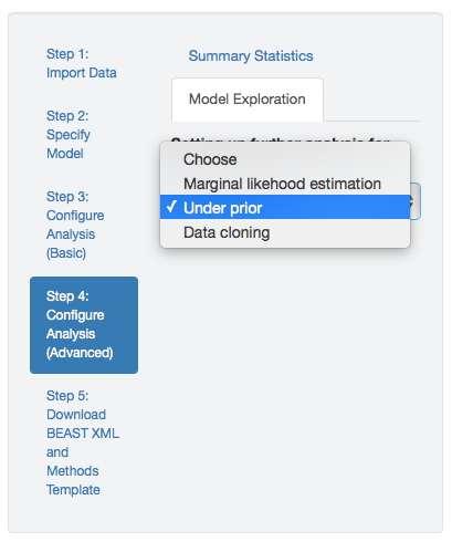
Figure 1.10: Set up an MCMC simulation to infer the joint prior probability distribution.
1.3.2 Robust Bayesian inference
Robust Bayesian inference explores the impact of prior specification on posterior estimates; it assesses the ‘robustness’ of our posterior estimates to prior specification. To perform this inference, first specify BEAST discrete-geographic analyses (following the instruction in the analysis-setup section) to estimate the joint posterior distribution using identical model but with different priors. To assess whether the posterior estimates are robust to these alternative priors, PrioriTree reads in BEAST output files to generate plots that depict the inferred posterior distributions of a given parameter under different priors.
Step 1: Importing BEAST log files
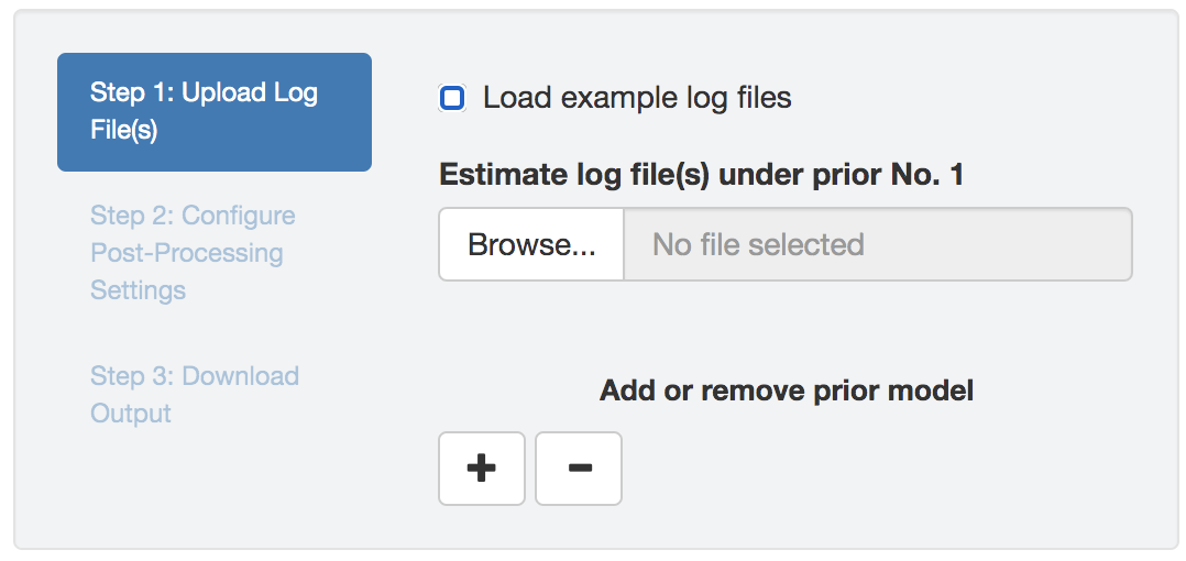
Figure 1.11: Initial panel: uploading log files.
Upload one or multiple (replicate MCMC simulations) BEAST log files (that contain parameter estimates under a given model and prior combination) to each input field; different input fields correspond to different priors (Figure 1.11).
These parameter log files can include samples from the joint posterior distribution (i.e., estimates with data) and/or samples from the joint prior distribution (i.e., estimates without data).
PrioriTree assumes that the uploaded log files are based on analyses of input files generated using PrioriTree; i.e., summaries of robust Bayesian analysis will only include log files with _underprior or _posterior as part of their name strings (other uploaded files are ignored).
Check the Load example log files box to load example log files to PrioriTree.
Selecting the parameter to examine
Once the log files have been successfully uploaded, PrioriTree will find the intersection of parameters (column names), which will then be displayed as shown in Figure 1.12: the focal parameters (i.e., the parameters that are commonly of interprets in empirical studies), if then exist, will be listed as radio buttons; choose the show others option to reveal the remaining parameters in a drop-down menu.
Simultaneously, when the parameter-selection panel appears, the start-processing button will also be enabled; clicking this button triggers the computationally demanding log-parsing routine.
Note that only a single parameter can be selected (either one of the radio buttons or one item from the drop-down menu); if you subsequently select another parameter to examine, the start-processing button will be reenabled and the log-parsing step will need to be re-executed.
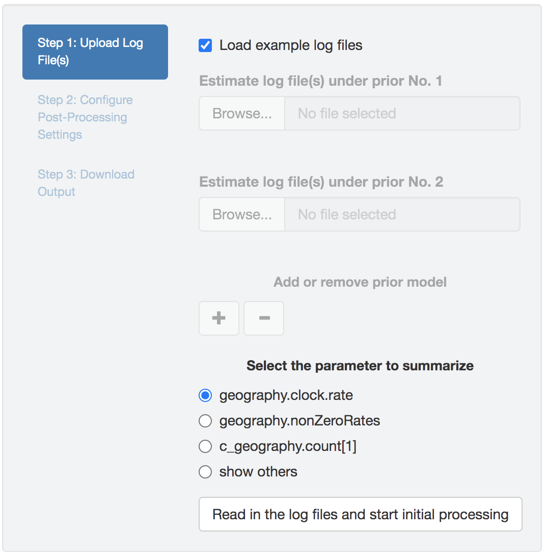
Figure 1.12: Select the parameter to examine.
Step 2: Configuring post-processing settings
Once PrioriTree finishes parsing the log files, two main panels will be enabled: the processing-setting panel (left) and the result-visualization panel (right). All the operations under this section should be computationally inexpensive so that the changes to the figure and/or table will appear more or less immediately.
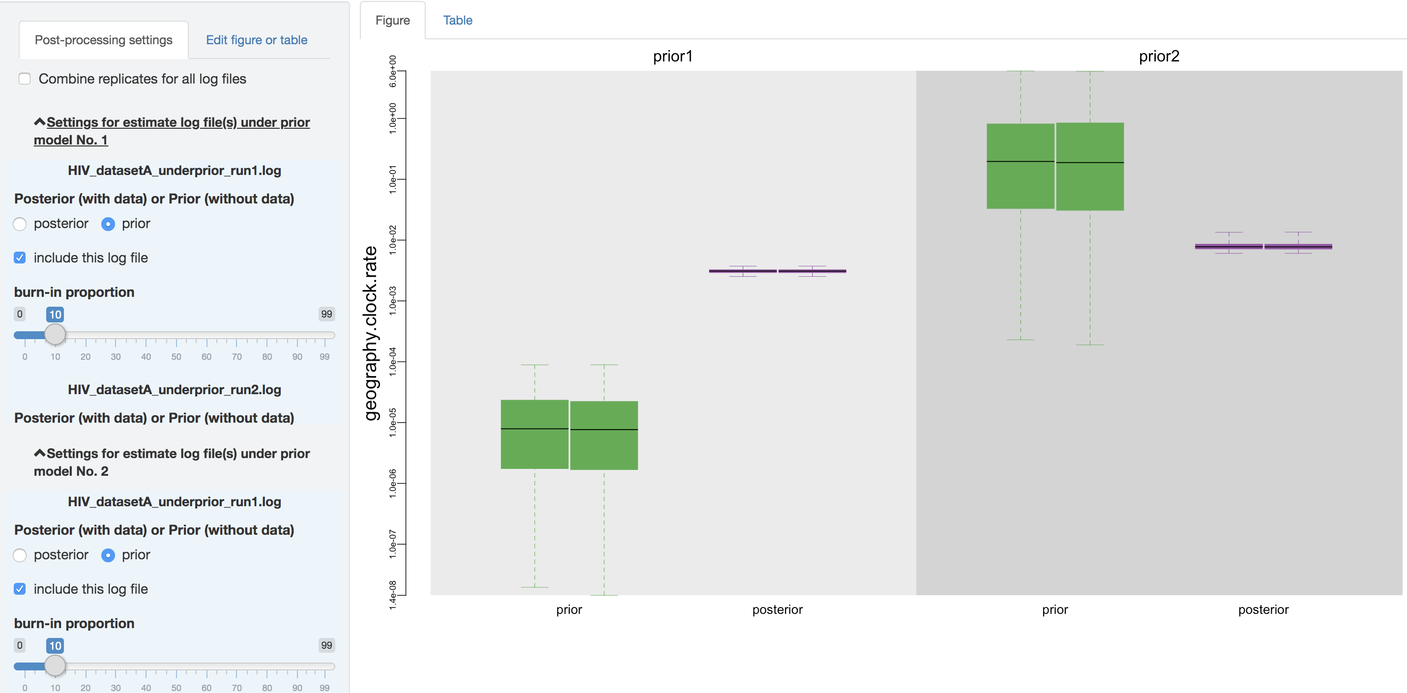
Figure 1.13: Configure post-processing settings.
Specifying output settings
Within the processing-setting panel, a separate scrollable collapsible subpanel is displayed under each prior model; each repeated chunk within that subpanel corresponds to the settings you can adjust for each log file (led by the log file name). With the first item (as radio buttons), you may adjust (if it has not been guessed incorrectly by PrioriTree) whether the given parameter log file was sampled from the joint posterior distribution or the joint prior distribution.
The second item allows you to exclude some log files without having to re-execute the log-parsing step. For instance, you may desire to compare the estimated posterior and prior distributions under each prior model in the first place, which may indicate the sensitivity of posterior estimates to the specified prior model. Then if you only want to present the comparison between the estimated posterior distribution, you can uncheck the log files for the estimated prior distribution.
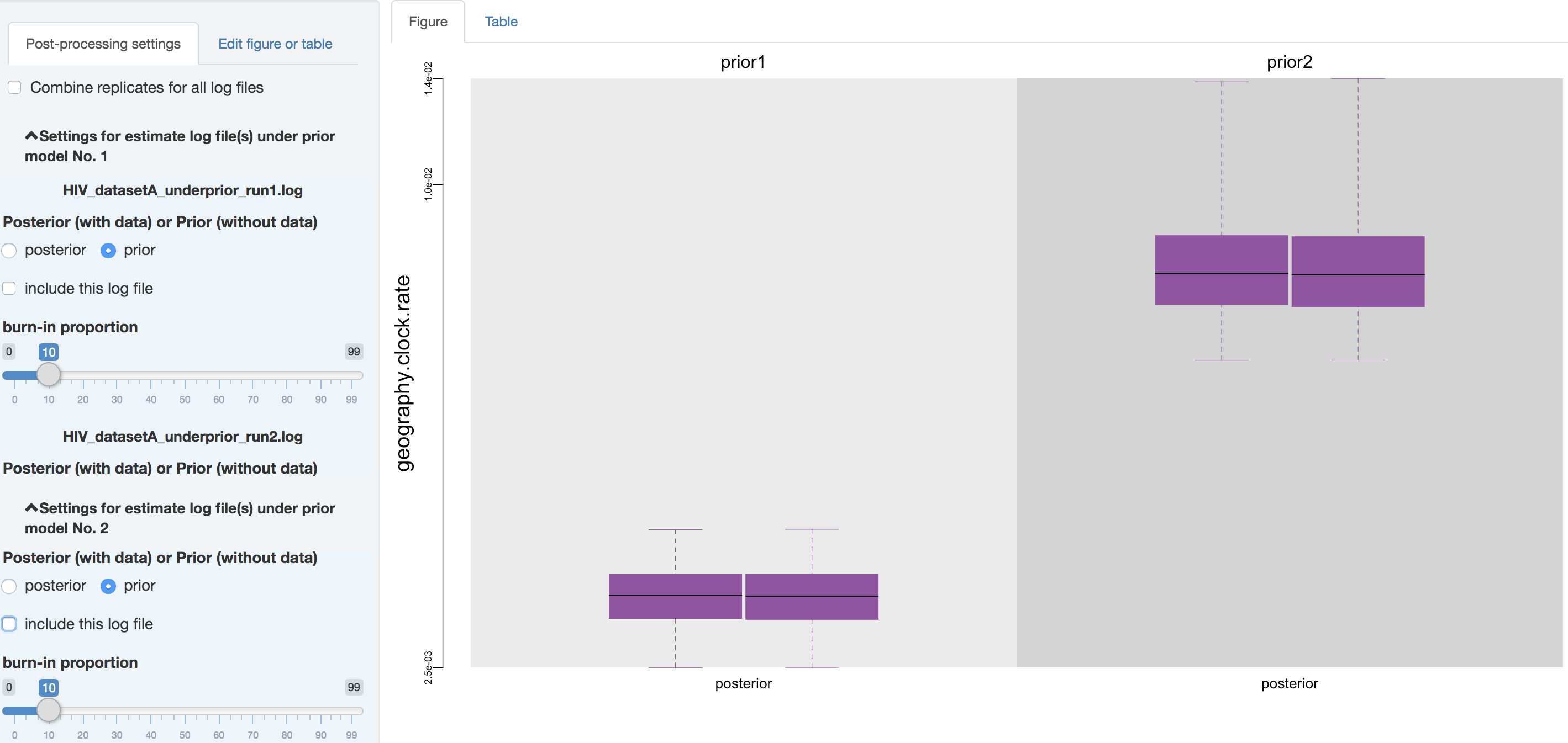
Figure 1.14: Exclude the prior estimates.
You can also adjust the burnin proportion of each log file independently using the slider object. You may also choose to combine all of the replicate log files (i.e., estimates under identical model and prior specification but sampled from independent MCMC simulations) using the check box on the top of the post-processing panel, after assessing whether the replicate MCMCs have converged.

Figure 1.15: Combine analysis replicates.
Editing figures
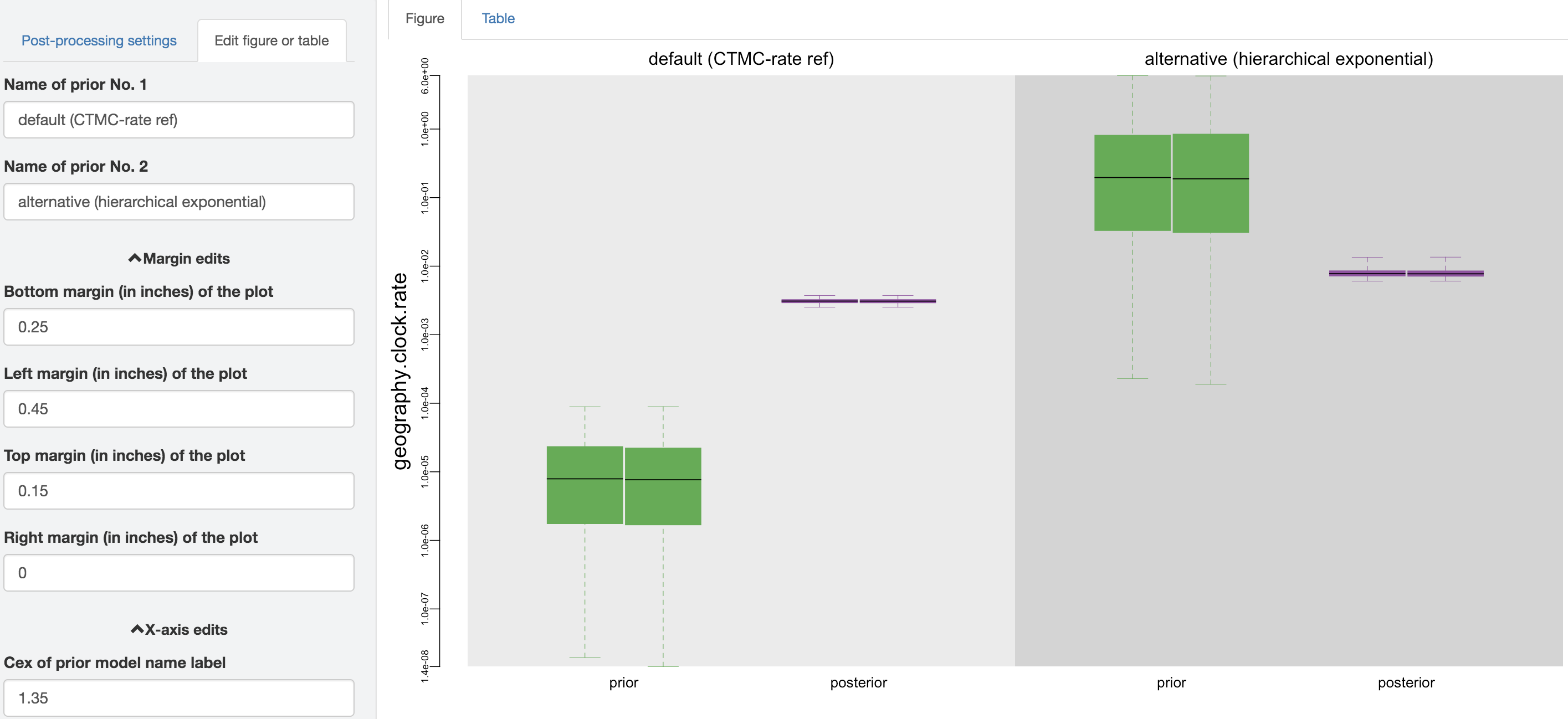
Figure 1.16: Edit figure.
You can make esthetic changes to the figure and/or table before saving the corresponding file. The fields under the figure-edit panel provide flexibility in modifying the appearance of the figure. You can view the exact values of the mean and \(95\%\) credible interval of each log file under the table tab.
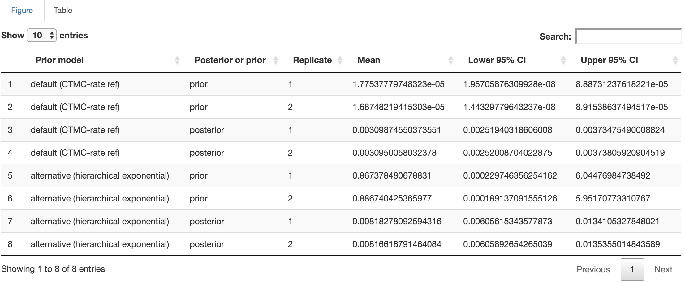
Figure 1.17: Distribution-summary table.
1.3.3 Data cloning
We can also assess the prior sensitivity of our biogeographic inferences using an approach called data cloning (Robert 1993; Lele, Dennis, and Lutscher 2007; Jose Miguel Ponciano et al. 2009; José Miguel Ponciano et al. 2012). PrioriTree provides functions that allow you to generate XML files with a series of clone numbers (that you can subsequently analyze using BEAST), and also includes functions that allow you to visualize the results of your data-cloning experiments.
Specifying data-cloning analyses
You can generate XML files using PrioriTree that specify the number of data clones.
Effectively, PrioriTree duplicates your original geographic data (i.e., the area in which each tip was sampled).
So, specifying \({k}\) clones will generate an alignment with \({k}\) copies of the original site; e.g., setting \({k = 5}\) will generate an alignment with 5 sites' that are identical copies of the original, singlesite’ (i.e., with an identical distribution of areas across tips).
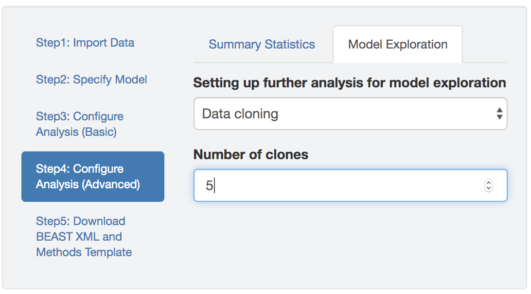
Figure 1.19: Specify BEAST data-cloning analyses.
After generating XML files that specify a series of data-cloning analyses (e.g., with 5, 10, 20 copies of the original data), run each XML file with BEAST. You may set up a series of data clones for a single choice of prior (e.g., to assess the proximity of the prior mean to the maximum-likelihood estimate (MLE) for a given parameter), or you may set up a series of data clones for two or more candidate priors (e.g., to assess the relative rate of convergence to the MLE under different priors for the parameter). PrioriTree provides features to help you explore the results of your data-cloning experiments—by generating plots of the marginal posterior probability distributions under different clone numbers and/or priors—which we describe below.
Summarizing data-cloning analyses
PrioriTree assumes that you have performed a sequence of BEAST analyses with increasing number of copies of the data using identical model (under one or multiple priors). PrioriTree takes the resulting BEAST output files as input to generate plots depicting the inferred distributions under various numbers of data clones (as well as under different priors if they exist).
Step 1: Import log files
Figure 1.20: Initial panel: uploading log files.
Upload multiple (from analysis replicates and/or under different number of clones) BEAST log files (that contain parameter estimates under the a given model and prior combination) to each input field; different input fields correspond to different priors (Figure 1.20).
These log files may include the estimates sampled from data-cloned distributions (with various numbers of copies of the data), the joint posterior distribution (one copy of the data), or the joint prior distribution (zero copy of the data).
PrioriTree assumes that the uploaded log files are produced using BEAST XML scripts generated by itself; i.e., for summarizing data-cloning analysis, upload log files with _datacloning, _posterior, or _underprior in their name strings.
Check the Load example log files box to load example log files to PrioriTree.
The following workflow of summarizing data-cloning analysis is effectively identical to the corresponding steps in the robust Bayesian analysis section.
Select the parameter to examine
Once the log files are successfully uploaded, PrioriTree finds the intersection of parameters (column names), and then displays them in the way shown in Figure 1.21: the focal parameters (i.e., the parameters commonly focused by empirical studies), if exist, will be listed as radio buttons; choose the show others option to reveal the remaining parameters in a drop-down menu.
Simultaneously, when the parameter selection panel appears, the start-processing button will also be enabled; clicking this button triggers the computationally demanding log-parsing action.
Note here only a single parameter can be selected (either one of the radio buttons or one item from the drop-down menu); if later you select another parameter to examine, the start-processing button will be enabled again and the log-parsing step needs to be re-executed.
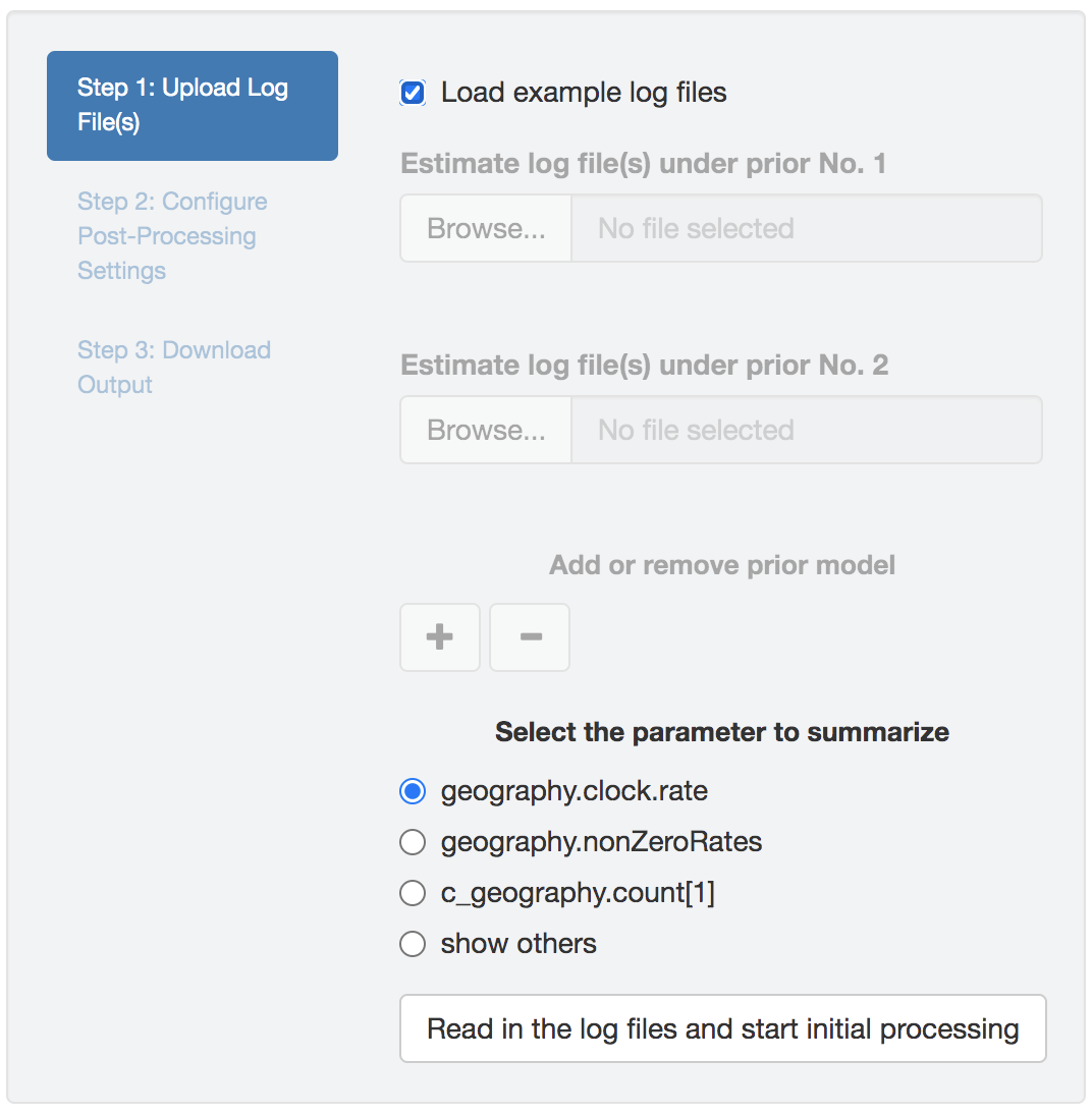
Figure 1.21: Select the parameter to examine.
Step 2: Configure post-processing settings
Once PrioriTree finishes parsing the log files, two main panels will be enabled: the processing-setting panel (left) and the result-visualization panel (right). All the operations under this section should be computationally inexpensive so that the changes to the figure and/or table should be seen immediately.
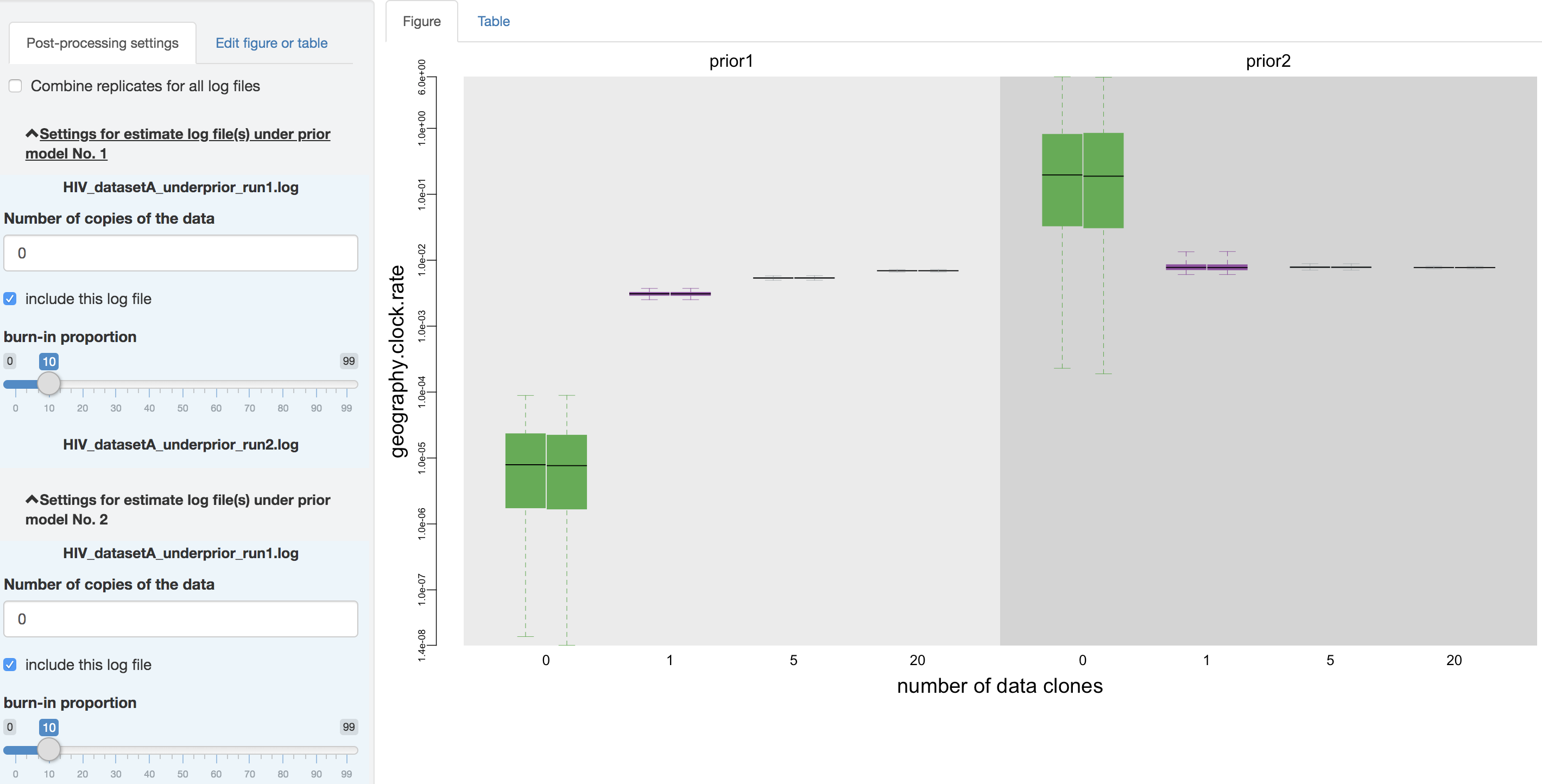
Figure 1.22: Configure post-processing settings.
Output processing settings
Within the processing-setting panel, a separate scrollable collapsible subpanel is displayed under each prior model; each repeated chunk within that subpanel corresponds to the settings you can adjust for each log file (led by the log file name). With the first item (as radio buttons), you may adjust (if it has not been guessed incorrectly by PrioriTree) whether the given parameter log file was sampled from the joint posterior distribution or the joint prior distribution. The second item allows you to exclude some log files without having to re-execute the log-parsing step.
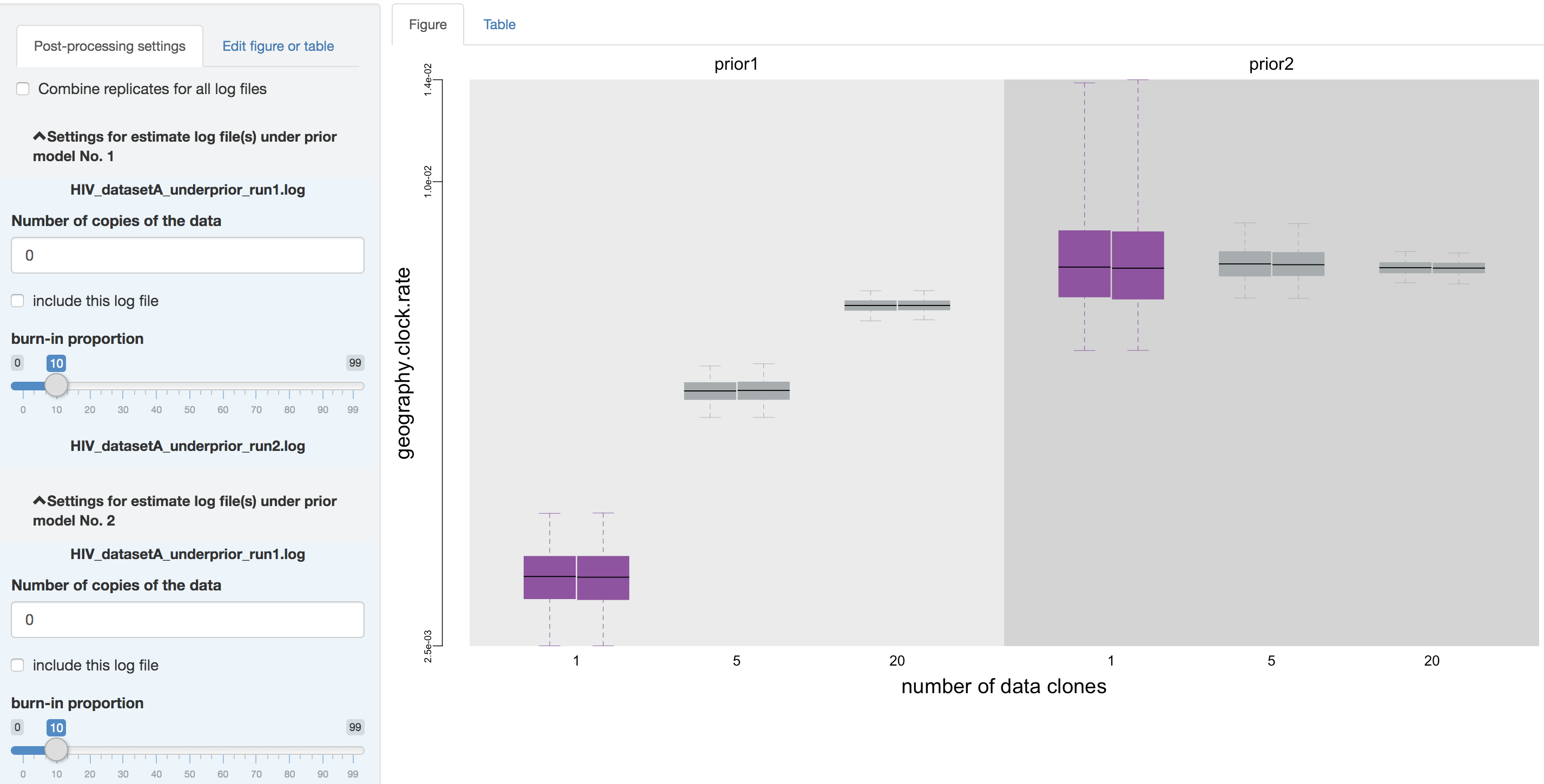
Figure 1.23: Exclude the prior estimates.
Thirdly, you can adjust the burnin proportion of each log file independently using the slider object. Also, you may choose to combine all the replicate log files (i.e., estimates under identical model and prior specification but sampled from independent MCMC chains) using the check box on the top of the post-processing panel, once confirming that the replicate MCMCs have converged.
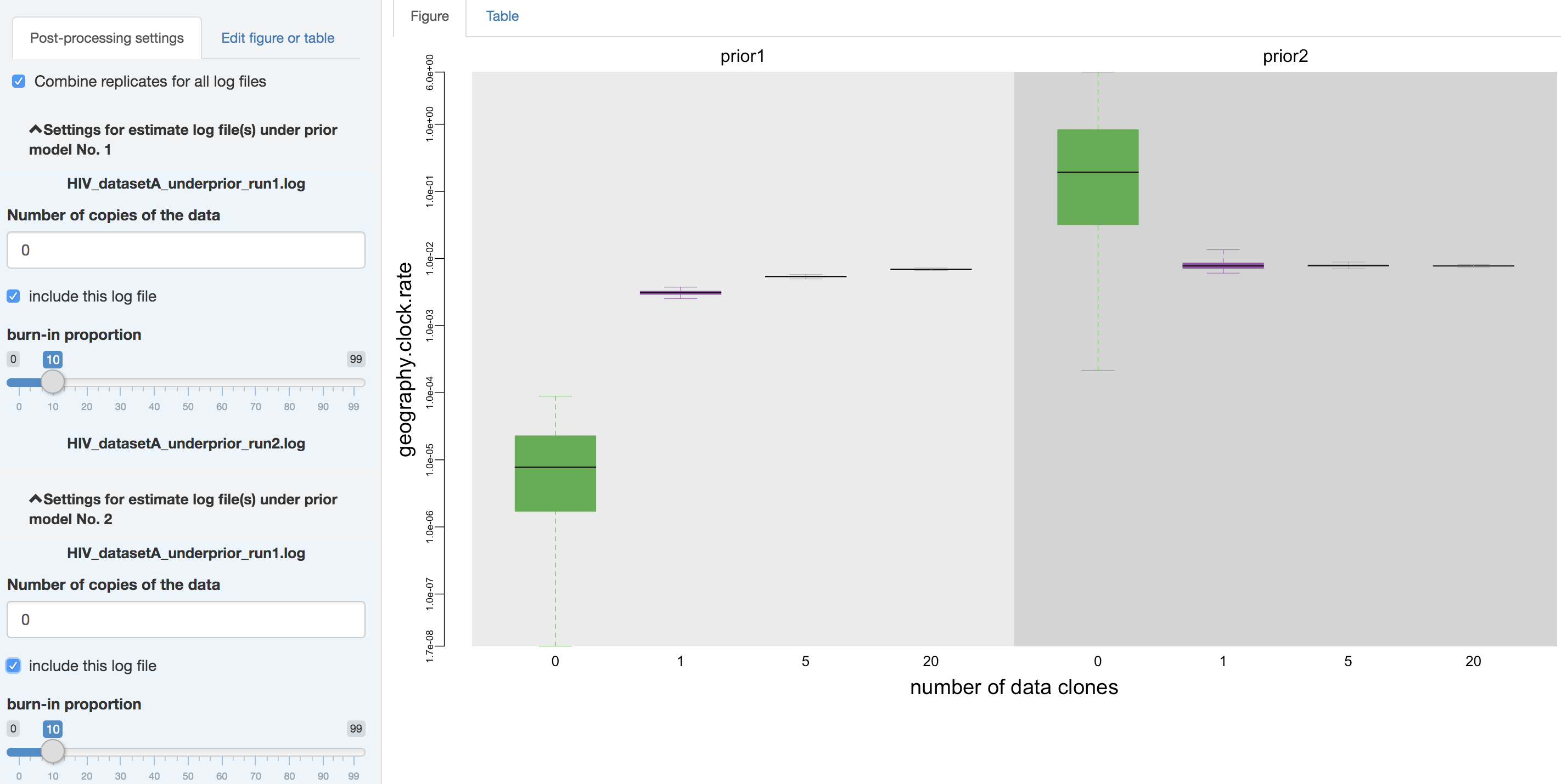
Figure 1.24: Combine analysis replicates.
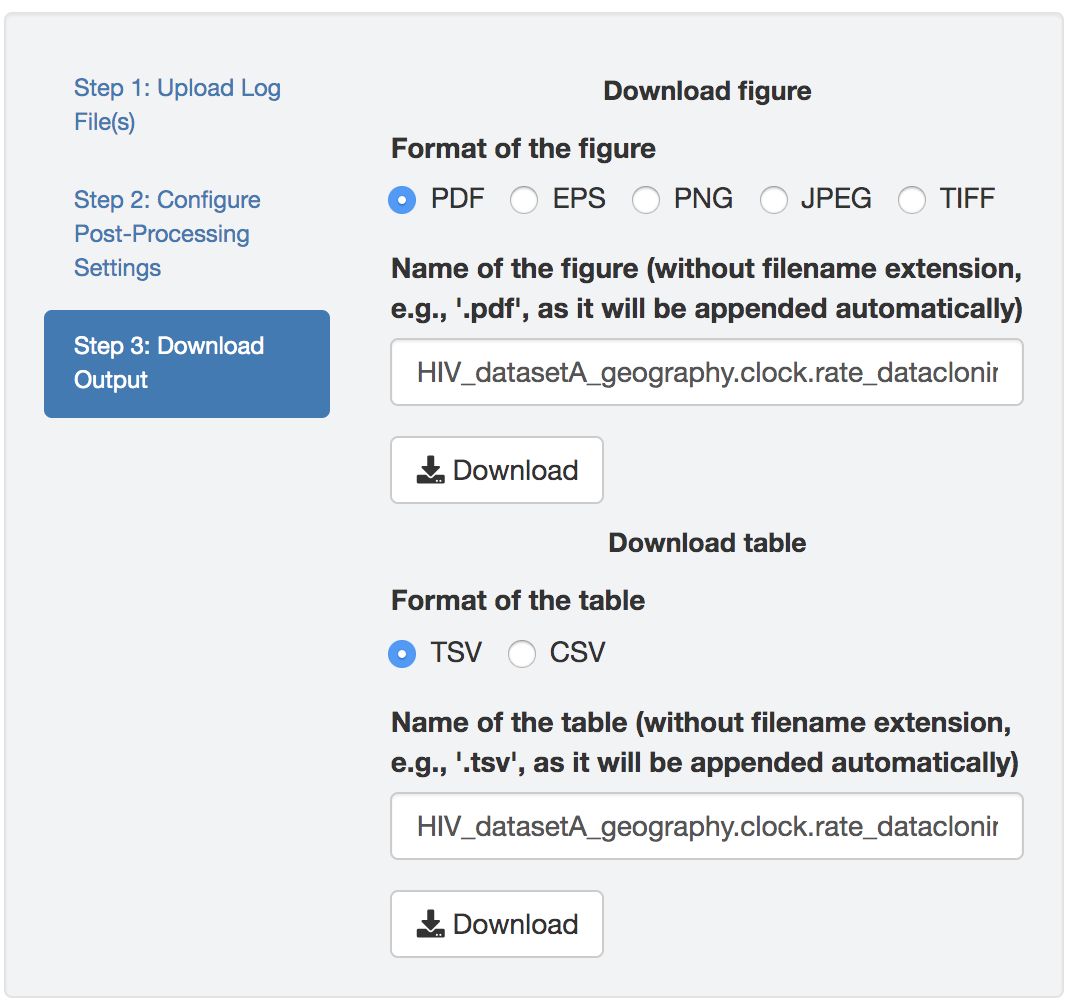
Figure edits
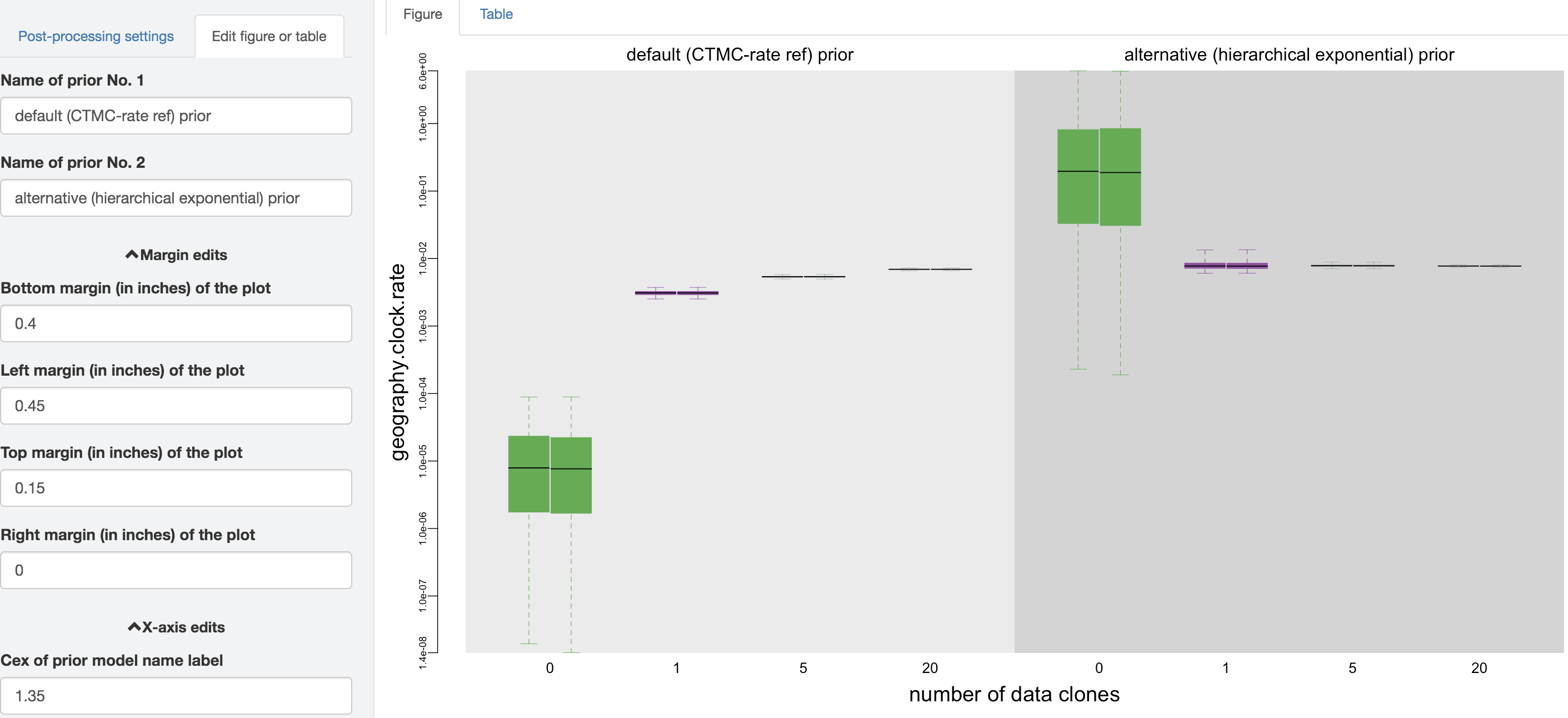
Figure 1.25: Edit figure.
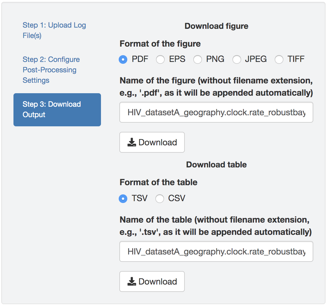
You may perform further cosmetic edits to the figure and/or table before saving them. The fields under the figure-edit panel provide flexibility in modifying the appearance of the figure. You can view the exact values of the mean and \(95\%\) credible interval of each log file under the table tab.
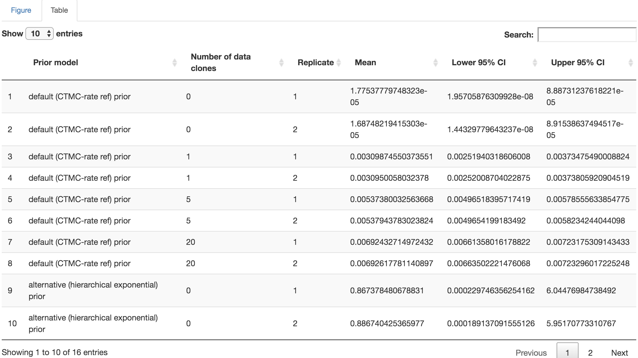
Figure 1.26: Distribution-summary table.