1.2 Interactively Specify BEAST Discrete-Geographic Phylodynamic Analyses Using Graphs of Priors
Here, we explain how to use PrioriTree to specify a basic BEAST discrete-geographic phylodynamic analysis with a focus on prior specification.
This basic analysis infers the discrete-geographic model parameters and the ancestral areas at internal nodes of the phylogeny.
The functionality described in this section is provided in the Analysis Setup main panel of the program.
See Section Detailed Guide for more detailed explanations of how to specify alternative models and priors, and how to set up further analyses (e.g., inferring the number of pathogen dispersal events between epidemic areas).
1.2.1 Step 1: Loading input files
PrioriTree requires two input files: one containing the discrete-geographic data, and the other containing the phylogeny (either a single summary tree or distribution of trees inferred from a previous analysis). Other panels (including the Methods Template Viewer and BEAST XML Viewer panels) in the PrioriTree interface will be enabled once both input files are uploaded (and pass the validity checks).
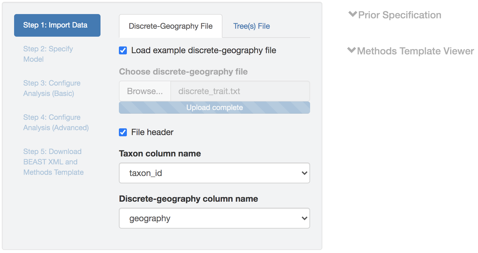
Figure 1.1: Import data panel (discrete-geographic data file).
Discrete-geographic data file
The geographic data file needs to be either a .csv or .tsv file that contains two (or more) columns.
The header (first row) of the file contains the names of the columns.
By default, PrioriTree assumes that the first column contains the species (pathogen-sample) names, and the second column contains the geographic area in which each species/pathogen was sampled.
If the columns in your data file are ordered differently, you can select the columns containing the species/pathogen name and geographic data from the drop-down menu after uploading the geographic-data file (other columns will then be ignored).
An example geographic-data file is available with the program; load it by checking the Load example discrete-geography file box.
The example geographic data file is also available here in the supplementary repository for Gao et al. (2022).
Tree file
The other input file contains the phylogeny to condition on (a single tree) or marginalize over (a distribution of trees) in the discrete-geographic phylodynamic analysis. This phylogeny is supposed to be inferred by previous analyses without using the geographic data. If the tree file contains more than one tree, then PrioriTree will specify the discrete-geographic BEAST analysis to average over this distribution of trees during the MCMC.
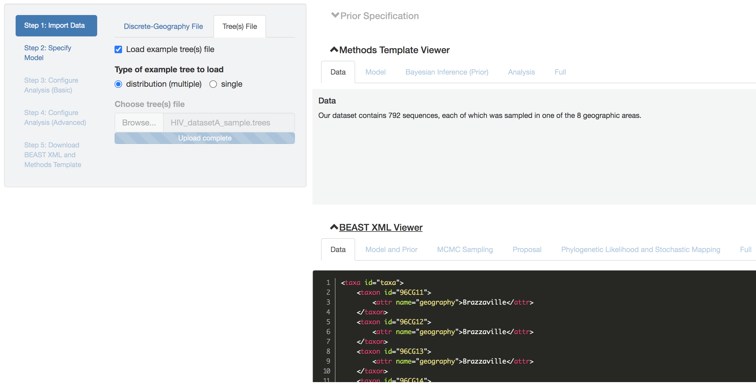
Figure 1.2: Import data panel (tree file).
See this for an example file that contains a single summary phylogeny, and this for an example file that contains a distribution of phylogenies.
Check the Load example tree(s) file box to load one of these example tree files to PrioriTree.
1.2.2 Step 2: Specifying model and configuring basic analysis
Now that input files have been read in, it is time to specify the discrete-geographic model.
Click the tab labelled Step 2: Specify Model (which won’t be clickable until both data files are uploaded).
Given that model and prior specification can have a large impact on discrete-geographic phylodynamic inferences, please go through this panel carefully to take advantage of the interactive and graphical features provided by PrioriTree for specifying model and priors.
Specifying model and priors
Discrete-geographic inferences are know to be very sensitive to the choice of model and prior specification. Below we briefly describe the basic steps for specifying the discrete-geographic model and priors; for details, see the detailed-guide section and Gao et al. (2022).
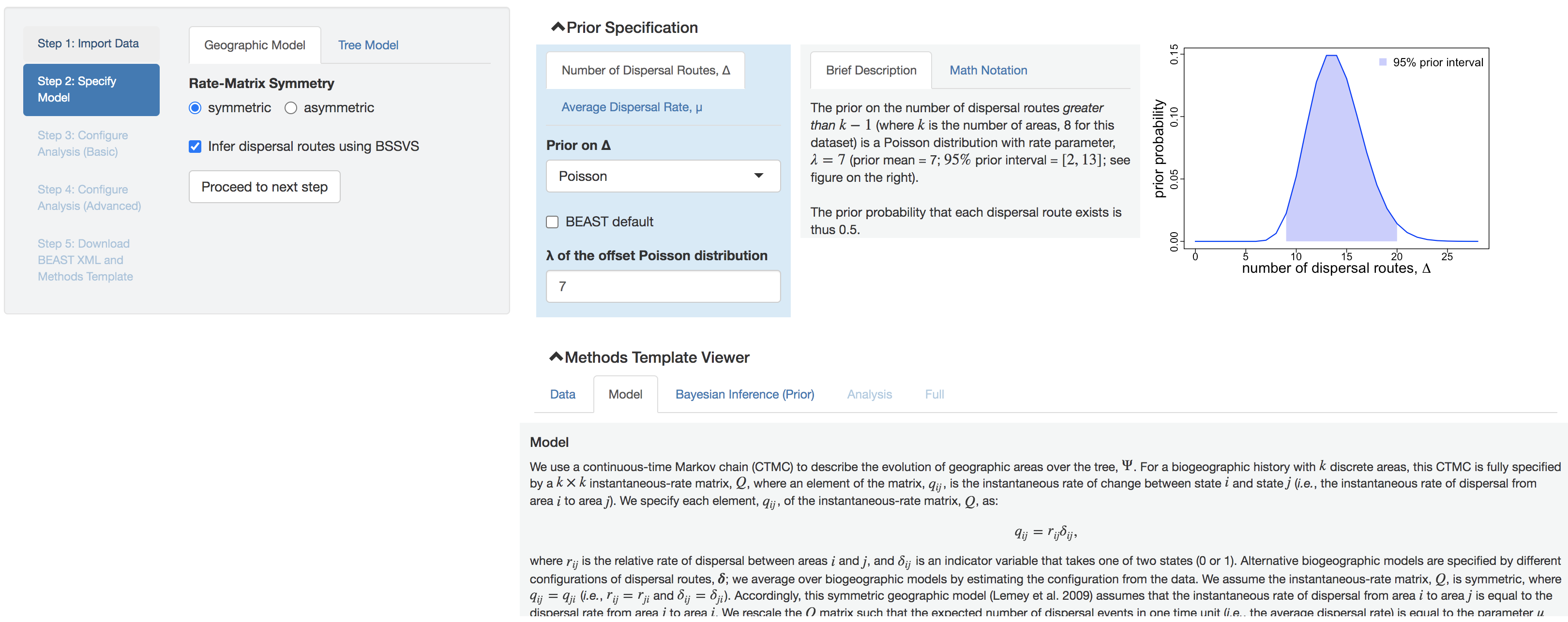
Figure 1.3: Model and prior specification panels.
Specifying model
Specify the discrete-geographic model (left panel) and choose the associated priors (right panel). Two tabs in this model-specification panel correspond to the geographic model and tree model, respectively.
In general, the tree-model part is not something to worry about. If the imported tree file contains only a single summary tree, it will be treated as a fixed variable in the inference; conversely, if the imported tree file contains a distribution of phylogenies, the default tree-model configuration should be appropriate.
In the geographic-model panel, there are two input fields:
Rate-Matrix Symmetry: the symmetric model assumes that the forward and backward dispersal rates between each pair of geographic areas are identical; the asymmetric model allows the forward and backward dispersal rates between each pair of geographic areas to differ.BSSVS: whether to use Bayesian Stochastic Search Variable Selection (BSSVS) to estimate the number of dispersal routes (see Lemey et al. (2009) and Gao et al. (2022) for detailed explanations).
Specifying priors
Priors may qualitatively impact the main biological conclusions drawn from discrete-geographic phylodynamic inferences (see Gao et al. (2022)).
The Prior Specification panel provides an interactive way to specify priors based on your biological knowledge before performing the analysis.
You can specify the prior distribution on each parameter (left subpanel) according to real-time feedback including the mathematical properties (middle subpanel) and visualization of the specified prior (right subpanel).
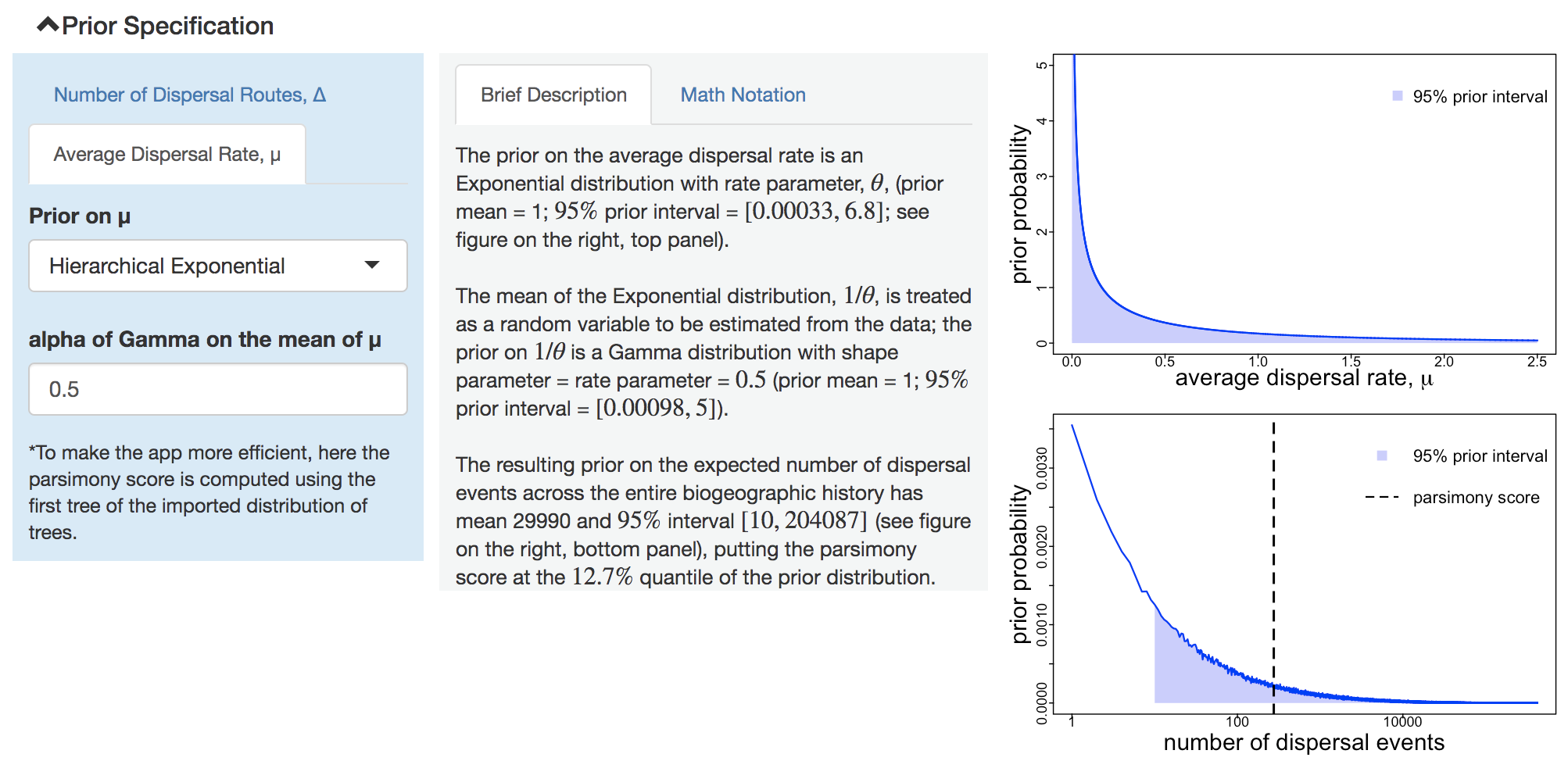
Figure 1.4: Specify prior on average dispersal rate.
Switch between the two parameters using the tabs in the left subpanel. For the prior on the average dispersal rate, PrioriTree plots both the average dispersal rate itself (top figure, right subpanel), as well as the resulting prior distribution on the number of dispersal events across the entire dispersal history (bottom figure, right subpanel). The vertical dashed line in the bottom figure indicates the parsimony score; you may use it as a reference to gauge whether a cosen prior is biologically sensible.
When using BSSVS, the dispersal-route indicators and their sum (the number of dispersal routes) will be part of the model; otherwise, these priors are not viewable.
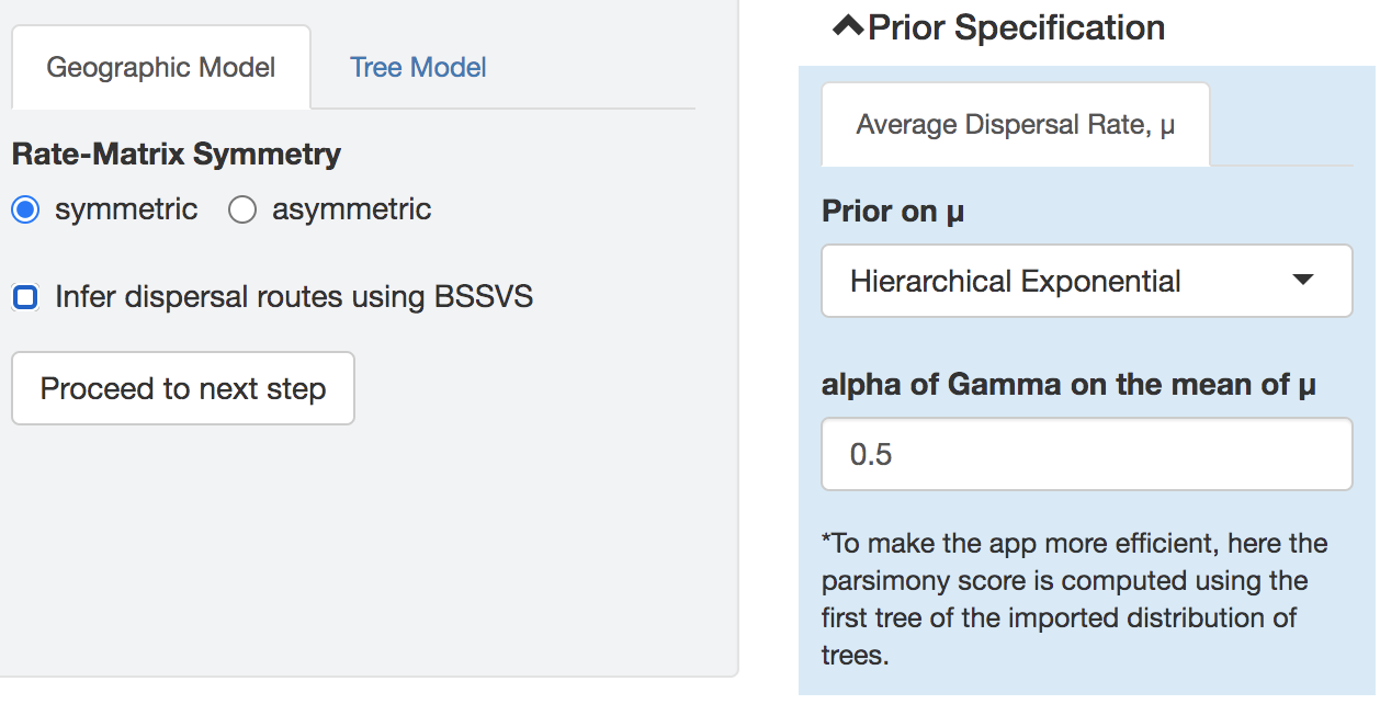
Figure 1.5: Prior specification panel when not using BSSVS.
Click Proceed to next step when you have completed specification of the model and priors.
A warning message will appear if none of the default settings have been changed.
If you intend to use the default settings, click Yes (otherwise make the desired changes to the model and/or priors).
This behavior applies to the remaining steps below.
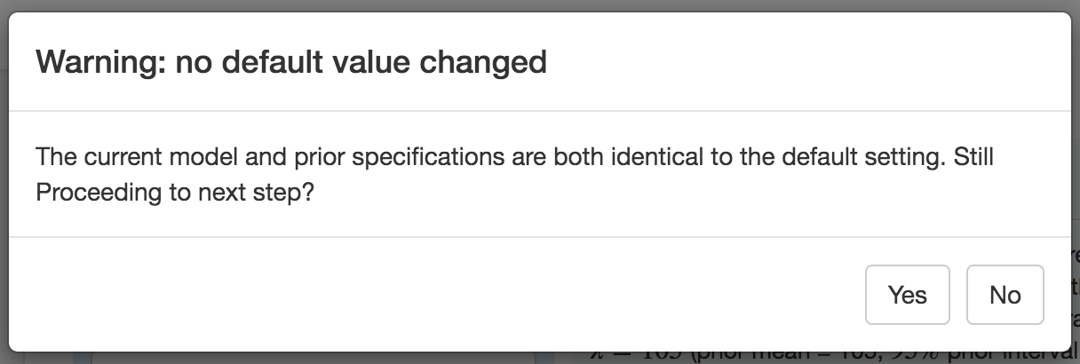
Figure 1.6: Warning message when no default settings has been changed.
1.2.3 Step 3: Specifying settings for basic analyses
Configure the MCMC settings of the BEAST analysis. The default settings of PrioriTree are likely to be appropriate for most discrete-geographic analyses. If the MCMC fails, you may want to increase the total number of generations (MCMC chain length) and/or adjust the proposal weights; see the detailed-guide section for detailed instructions.
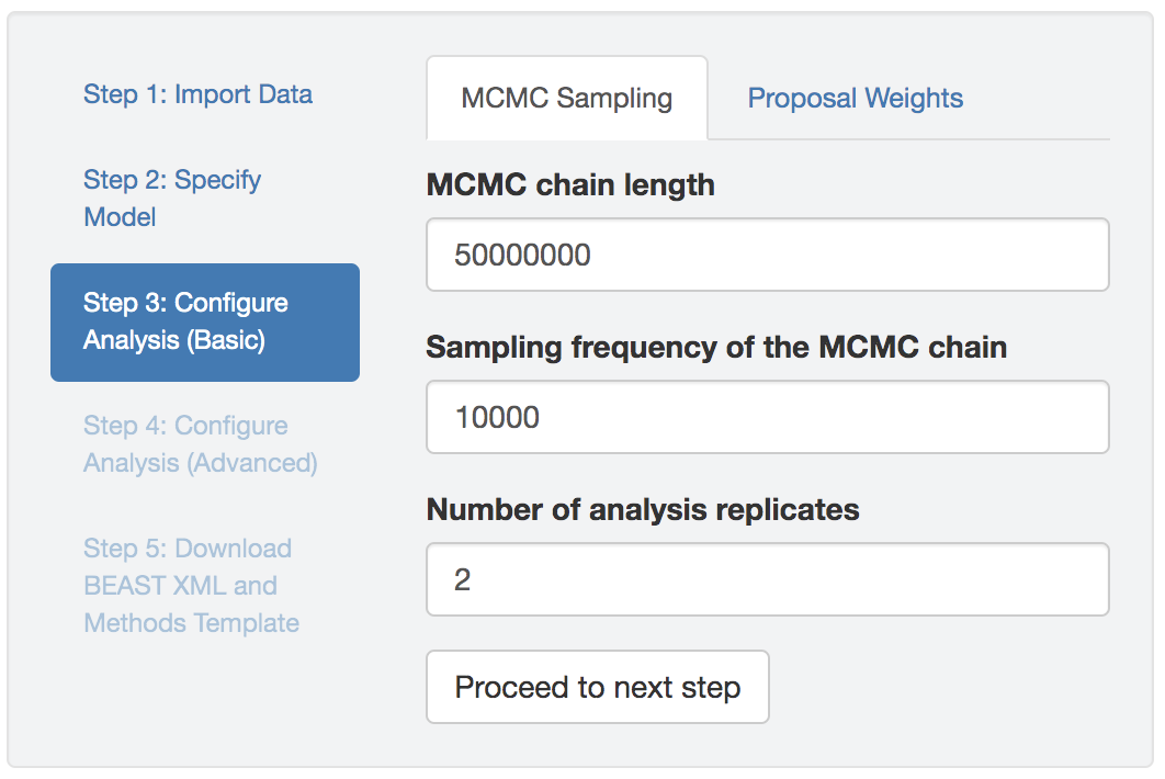
Figure 1.7: Basic analysis-setting configuration panel.
Brief explanation of the input fields:
- MCMC chain length: the total number of generations for the analysis;
- MCMC sampling frequency: the intervals (in terms of generations) that MCMC samples will be written to the log files, and;
- Proposal weight: the relative probability of performing each proposal
In addition, you may specify the number of replicate MCMC simulations using the third field of this panel. As MCMC is a numerical algorithm approximating the posterior distribution, it is necessary to run multiple MCMCs targeting the same distribution to assess the reliability of the posterior estimates; the default number of replicates is thus set to 2 (although 4–8 replicates are generally preferable, provided sufficient computational resources are available).
1.2.4 Step 4: Saving Output
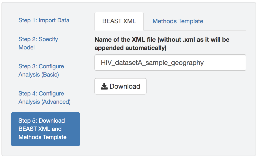
Figure 1.8: Download the BEAST XML script.
Download the BEAST XML script produced by PrioriTree. The default name of the XML script is generated by PrioriTree to indicate the type of analysis that you specified. If the inference involves averaging over a distribution of phylogenies (i.e., the imported tree file contains a distribution of trees), the tree file needs to be put in the same directory as the XML script for it to run. An example output XML scripts zipped folder is available here.
You may also download a text file that describes the model and prior specification, as well as the analysis configuration, to serve as a template for the methods section of your study. An example methods-description text file generated by PrioriTree is available here.
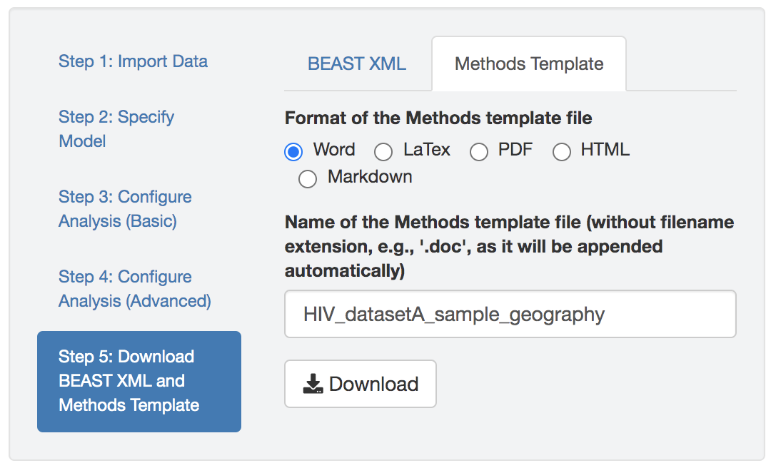
Figure 1.9: Downloading the Methods Description Text File