1.4 Assessing Model Fit
Model-based inference—including phylodynamic inference—assumes that our inference model provides a reasonable description of the process that generated our study data; otherwise, our inferences—including estimates of relative and/or average dispersal rates and any summaries based on those parameter estimates (ancestral areas, dispersal histories, number of dispersal events, etc.)—are apt to be unreliable. Additionally, comparing alternative discrete-geographic models provides a means to objectively test hypotheses regarding the history of dispersal (i.e., by assessing the relative fit of our data to competing models that are specified to include/exclude a parameter relevant to the hypothesis under consideration). PrioriTree implements functions to help you assess both the relative fit and absolute fit of discrete-geographic models to an empirical dataset.
1.4.1 Comparing the relative fit of competing models
PrioriTree allows you to set up marginal-likelihood BEAST analyses by appending a marginalLikelihoodEstimator section to the XML, after the analysis configuration section of the MCMC that approximates the joint posterior distribution; this will allows you to estimate marginal likelihood through both thermodynamic integration (Lartillot and Philippe 2006) and stepping-stone sampling (Xie et al. 2011; Baele et al. 2012).
The number of powers and how many MCMC generations under each power may impact the accuracy of the marginal-likelihood estimates; default values are likely to be sufficient for most empirical datasets and models. However, the most straightforward way to assess the reliability of marginal-likelihood estimates is to perform replicate analyses to ensure that estimates are stable across replicates analyses. If the estimates differ significantly among replicates (say greater than a few log-likelihood units, especially if it is equal to or greater than the difference between the log marginal-likelihood estimates under competing models), consider increasing the number of powers and/or the MCMC chain length under each power.
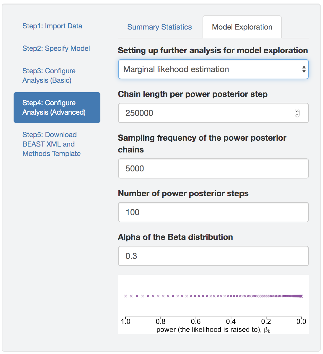
Figure 1.28: Marginal likelihood estimation analyses.
1.4.2 Posterior-predictive checking
To perform posterior-predictive checking, PrioriTree requires you to provide the observed data as well as the estimates (as log and tree files produced by BEAST) inferred from the data, assuming these inference outputs are generated by BEAST using the XML scripts produced by PrioriTree (only when this is the case, PrioriTree can reliably parse the log file and figure out the exact discrete-geographic model used in the inference, so that it can simulate data under that model). Once all the required input files are provided, you can start the simulation in PrioriTree, and then PrioriTree will generate plots to show the posterior-predictive distributions for each replicate analysis (as well as under different priors if they exist).
Step 1: Import files
Discrete-geographic data file
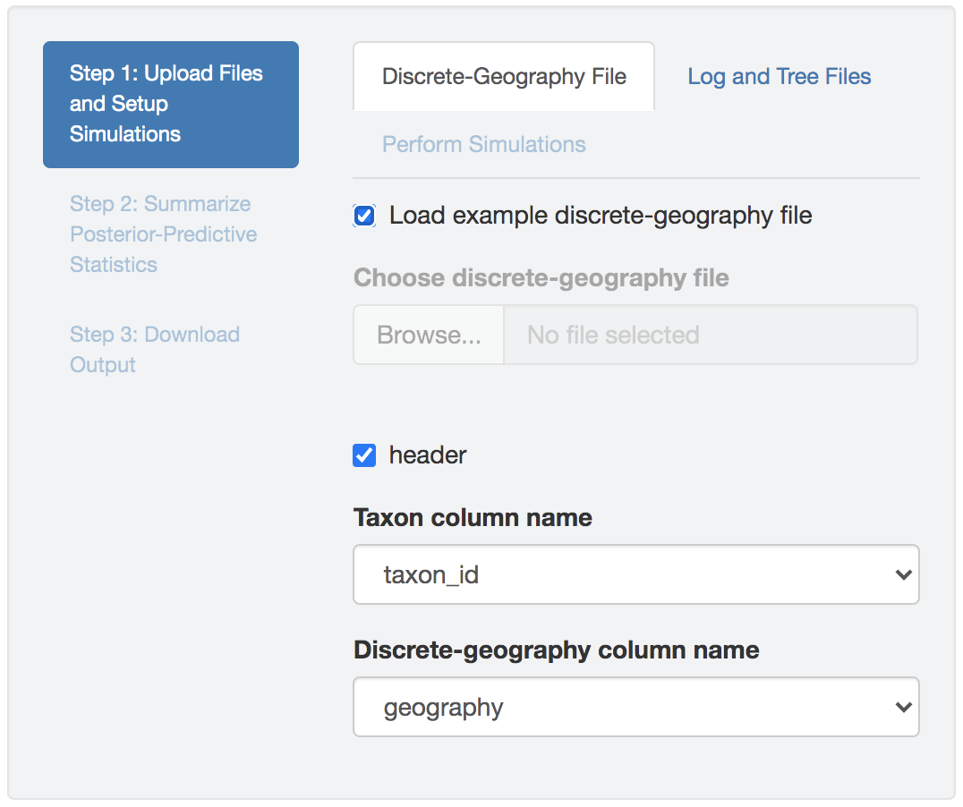
Figure 1.29: Import discrete-geographic data.
The discrete-geographic data file needs to be either a .csv or .tsv file that contains two (or more) columns.
The header (first row) of the file contains the column names.
By default, PrioriTree assumes that the first column contains the species/pathogen-sample names, and the second column contains the geographic area for that species/pathogen sample.
If the columns in your data file are ordered differently, select the columns containing the species/pathogen-sample name and geographic data from the drop-down menu after uploading the discrete-geographic data file into PrioriTree (the other columns are ignored).
Check the Load example discrete-geography file box to read in an example discrete-geographic data file.
Parameter log and tree files
Upload one or multiple (replicate analyses) BEAST log/tree files (that contain parameter estimates under the a given model and prior combination) to each input field; different input fields correspond to different priors. Note that you need to upload both the log file(s) and the corresponding tree file(s). To simulate a dataset, PrioriTree requires the tree and geographic-model parameters.
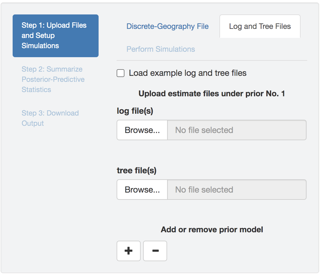
Figure 1.30: Upload BEAST output files.
PrioriTree assumes each sample in the log file and in its associated tree file match each other; i.e., they should have been sampled from the same iteration of a BEAST analysis (the default behavior when the XML scripts generated by PrioriTree were used).
If you have combined replicate analyses or have thinned their estimates files, identical operations need to be applied to both the log file and the associated tree file.
Check theLoad example log and tree files box to read in an example sets of log and tree files.
Performing posterior-predictive simulations
Once all the input files (including the geographic-data file, parameter log file(s) and the associated tree file(s)) are uploaded and that these files are valid (with correct and identical format across all files), the Perform Simulations tab will be enabled.
In the Perform Simulations panel, you can either choose to simulate a dataset using each sample in the uploaded distribution by checking the Perform one simulation for each sample box, or specify the desired number of simulated datasets by first unchecking the box and then editing the simulation-number field.
Finally, once the simulation configuration is complete, click the Start posterior-predictive simulation button to initiate the computationally demanding log-parsing and forward-simulation actions.
This simulation step may a while to complete; the timer required will scale with the number of sequences and number of geographic areas in the dataset, as well as the number of simulations that you specified.
If you later decide to change any of the uploaded files and/or the number of simulations, click the Start posterior-predictive simulation button to re-execute the simulation step.
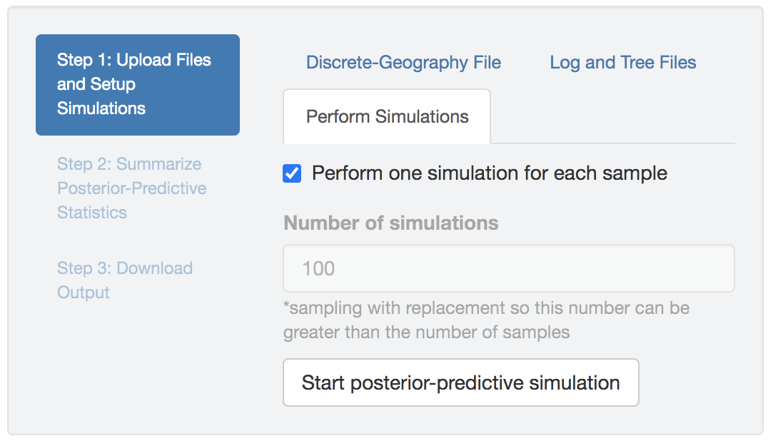
Figure 1.31: Start posterior-predictive simulations.
Step 2: Configuring post-processing settings
Once PrioriTree completes the posterior-predictive simulations, two panels will be enabled automatically: the processing-setting panel (left) and the result-visualization panel (right). All the operations under this section should be computationally inexpensive so that the changes to the figure and/or table appear immediately.
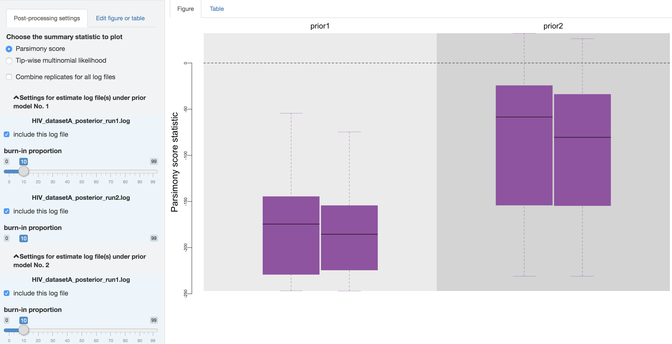
Figure 1.32: Configure post-processing settings.
Specifying output settings
First, you can choose to visualize the posterior-predictive distributions under one of the two available statistics: 1) parsimony statistic and 2) tip-wise multinomial statistic (see the theoretical-background section for details), and switch between them using the radio buttons on the top of the post-processing settings panel.
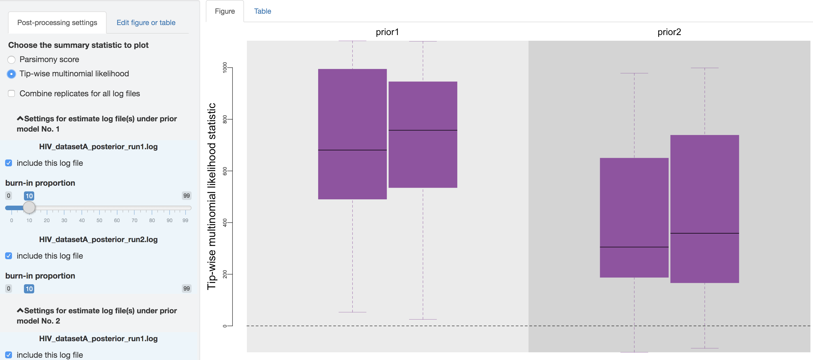
Figure 1.33: Posterior-predictive distributions of the tip-wise multinomial likelihood statistic.
There is a checkbox that you can click to combine all the replicate analysis (i.e., estimates under identical model and prior specification), once confirming that the replicate MCMCs have converged.
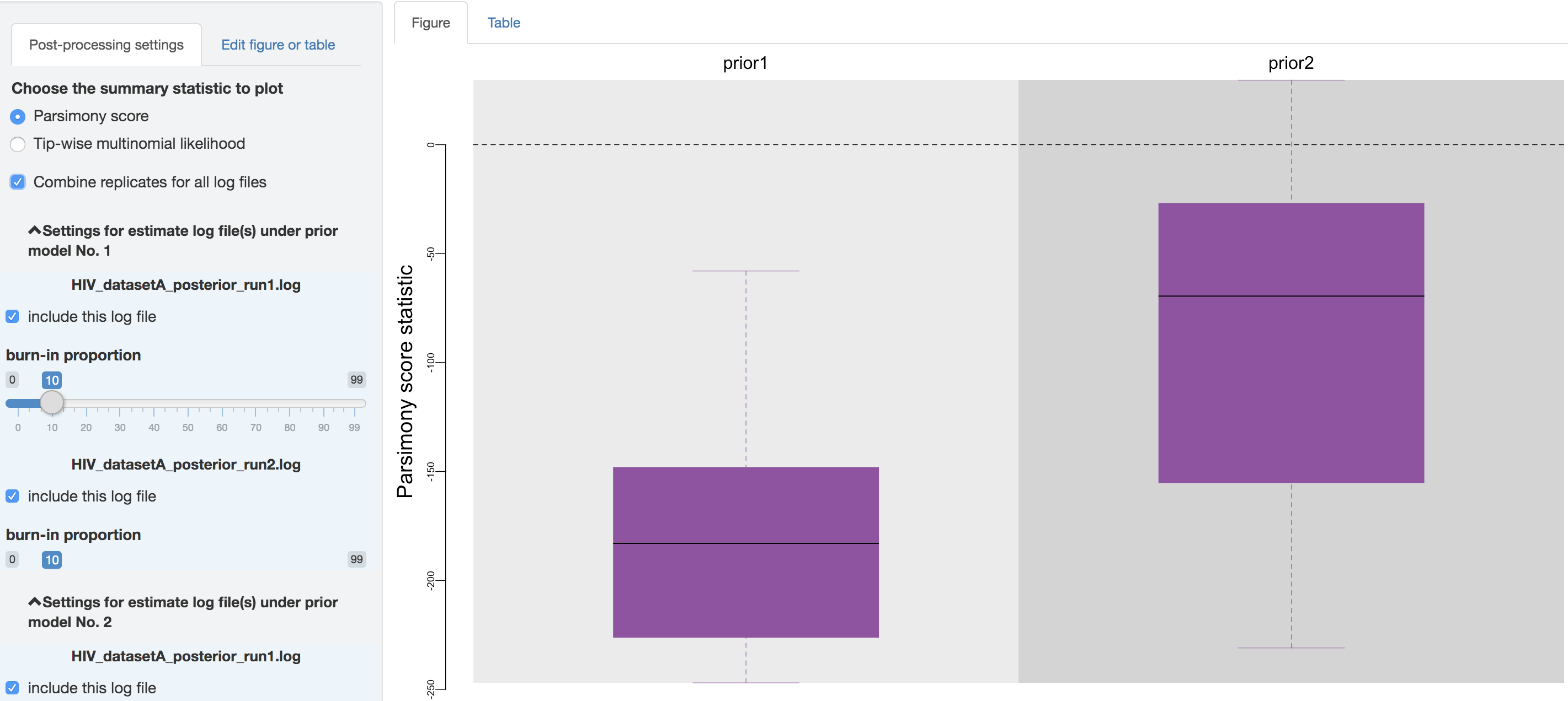
Figure 1.34: Combine replicates.
Below the checkbox, a separate scrollable collapsible subpanel is displayed under each prior model; each repeated chunk within that subpanel contains the settings you can adjust for each log file (led by the log file name). The first item allows you to exclude some log files without having to re-execute the log parsing step. With the second item, you can adjust the burnin proportion of each analysis independently using the slider object.
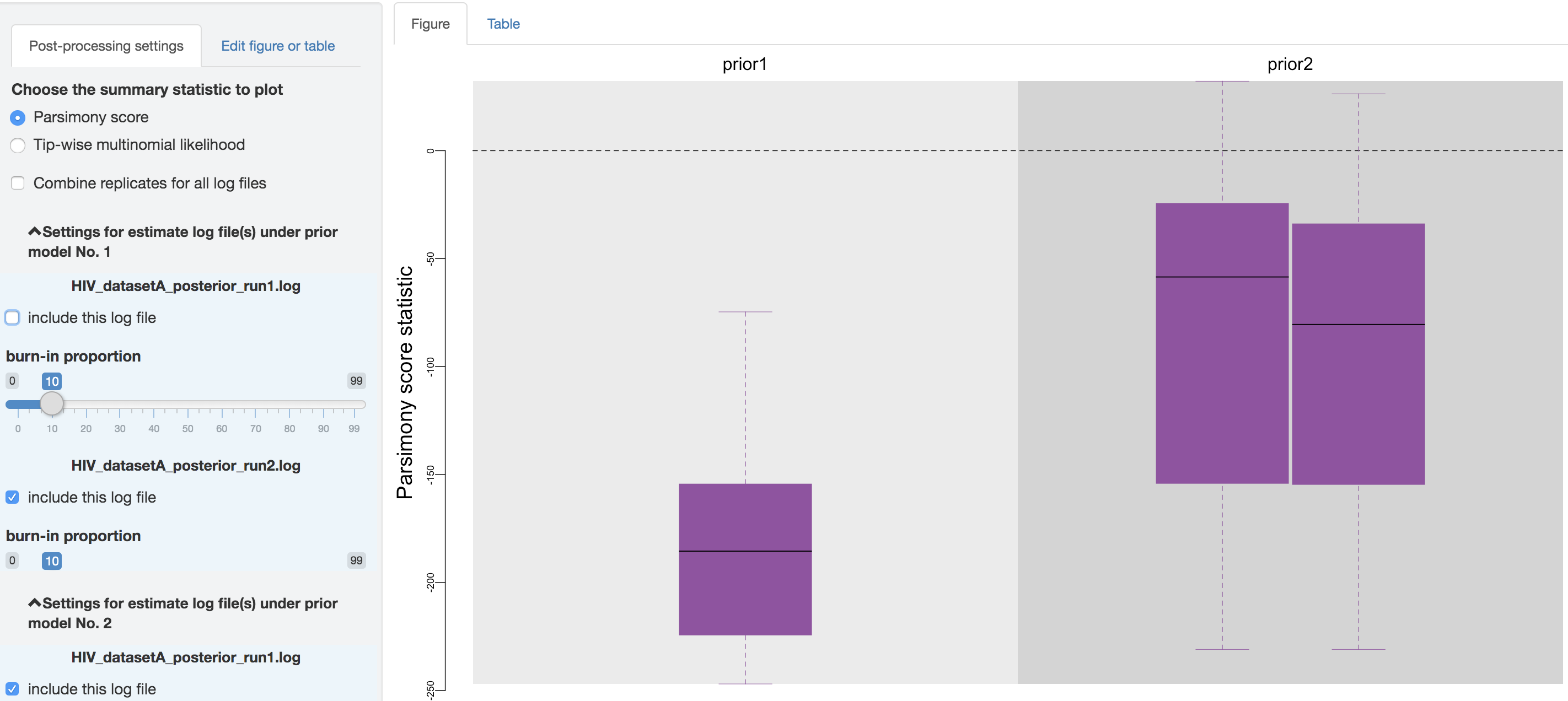
Figure 1.35: Exclude some log files.
Editing figures
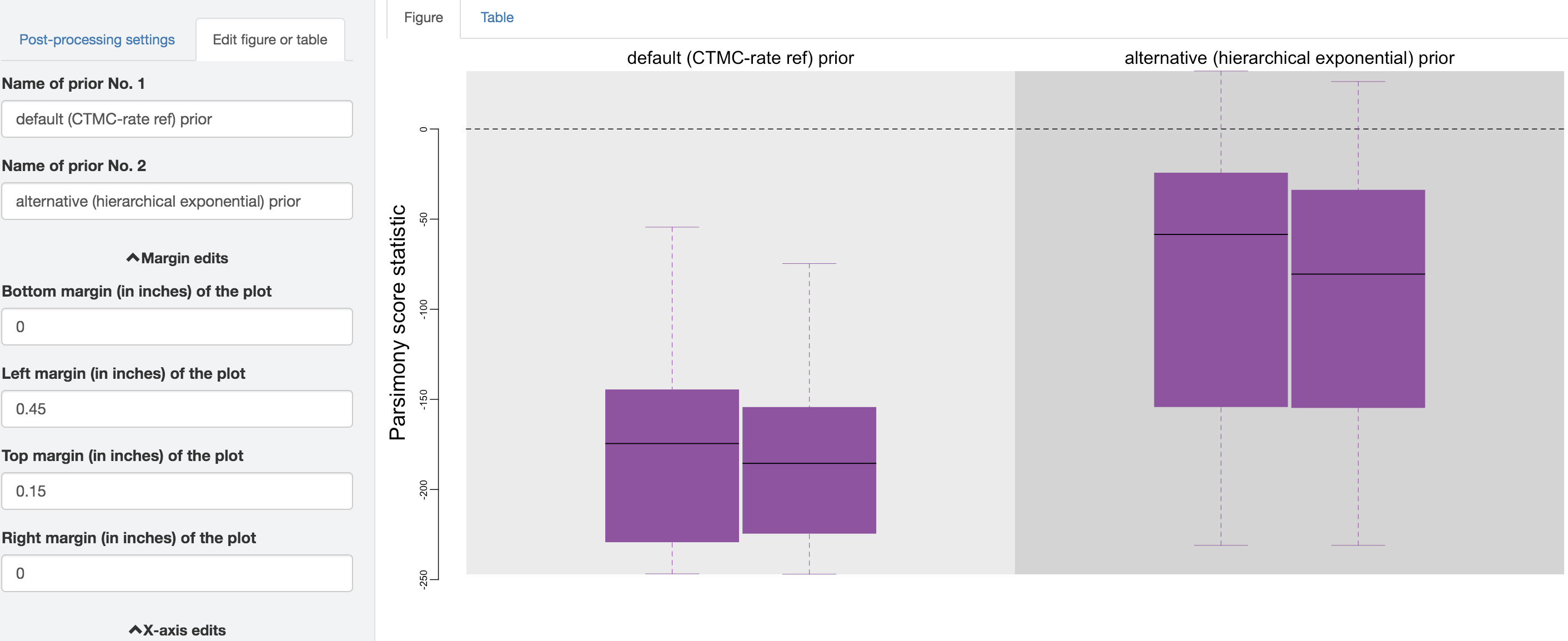
Figure 1.36: Edit figure.
You can make esthetic changes to the figure and/or table before saving these files. The fields under the figure-edit panel provide flexibility for modifying the appearance of the figure. You can also view the exact posterior-predictive p-values of each analysis for both statistics together under the table tab.
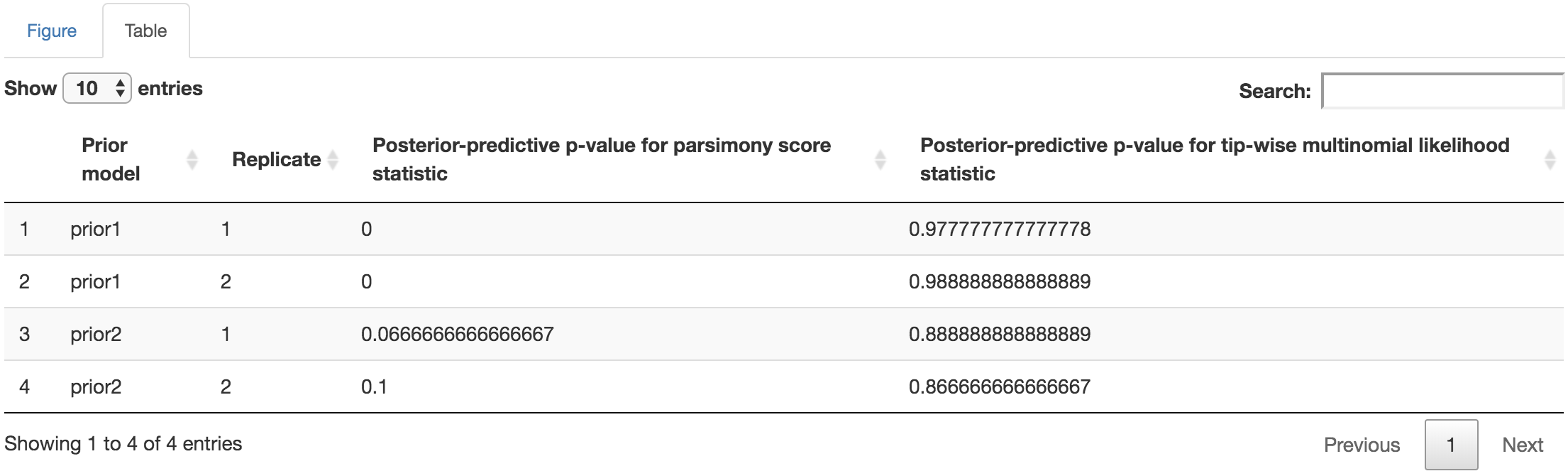
Figure 1.37: Posterior-predictive p-values table.
Step 3: Saving output files
Saving figure or table files
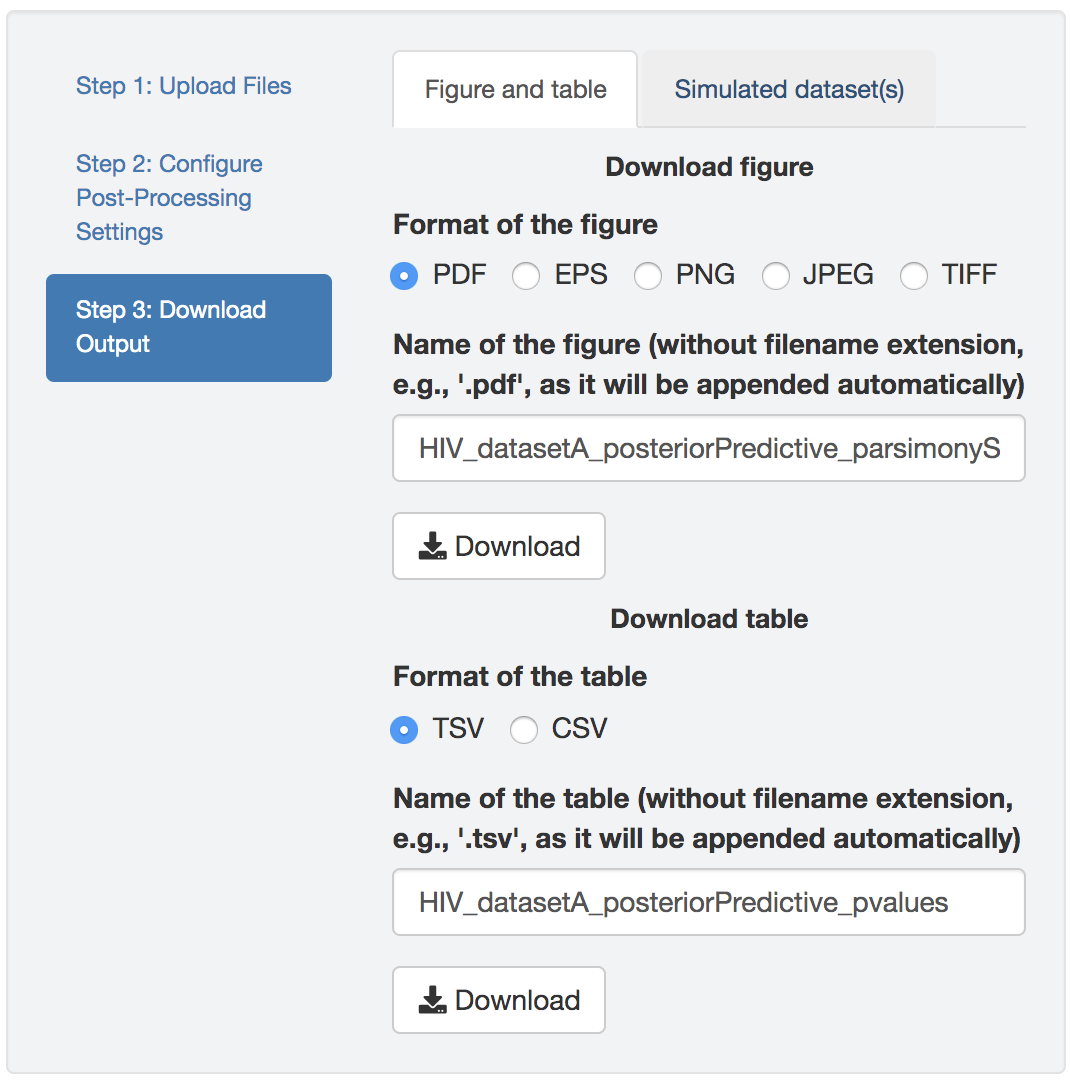
Figure 1.38: Download figure and/or table.
Finally, download the figure and/or the table in the desired format. The default figure/table name generated by PrioriTree indicates the type analysis and the selected posterior-predictive statistic (only for the figure as the table contains both statistics).
Saving simulated datasets
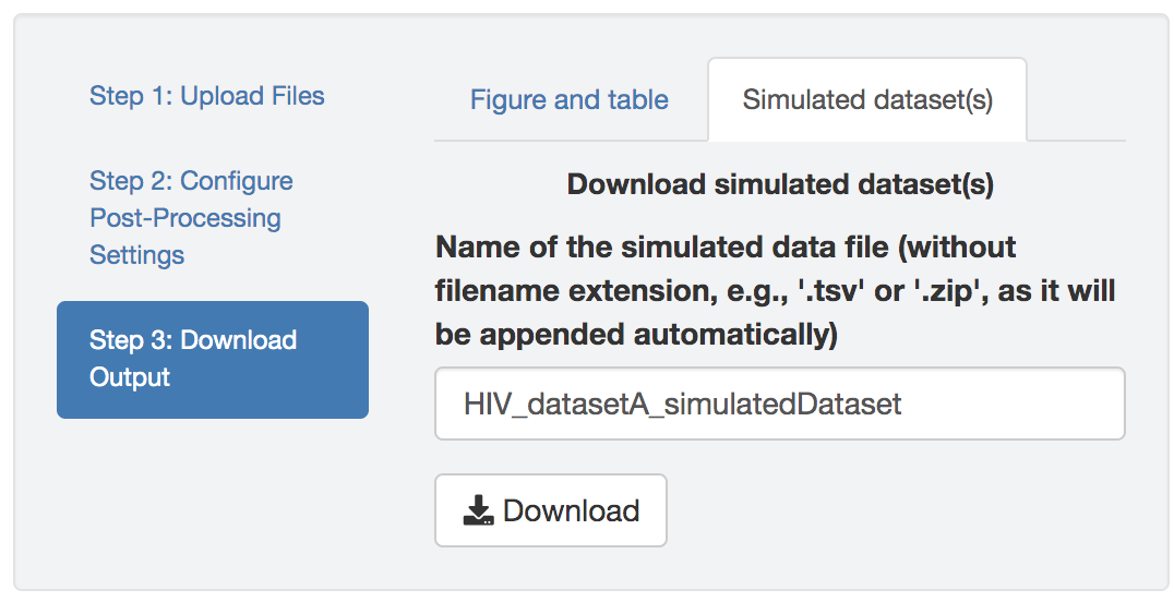
Figure 1.39: Download the simulated datasets.
You can also download the posterior-predictive simulated datasets and summarize them in other ways (e.g., using alternative summary statistics other than the two provided by PrioriTree).
For each analysis, PrioriTree simulates datasets (each contains state of every tip in the tree) and then writes them out as a single .tsv file, where each column indicates a tip (first row contains tip names as column names) while each row contains a simulated dataset (so the number of rows, after the first header row, is identical to the number of post-burnin samples of the corresponding analysis).
When there are multiple analyses (replicates and/or under different prior models), PrioriTree will produce a zipped folder that contains all the .tsv files (where each .tsv file contains the simulated datasets for the corresponding analysis).
The name of each .tsv file contains the prior model name as well as the replicate id as part of its string, so that you can match them with the uploaded analysis files.
A zipped example folder containing the simulated datasets is available here.