2.3 MCMC Settings
2.3.1 The Metropolis–Hastings Algorithm
Recall that Bayesian inference is focused on the joint posterior probability distribution of our model parameters. The posterior probability cannot be solved analytically, so we must resort to numerical methods to approximate the joint posterior probability. Here we briefly describe the numerical method used to estimate the joint posterior probability distribution of discrete-geographic model parameters in BEAST: the Metropolis–Hastings Markov chain Monte Carlo (MCMC) algorithm.
The Metropolis–Hastings algorithm (Metropolis et al. 1953; Hastings 1970) entails simulating a Markov chain that has a stationary distribution that is the joint posterior probability distribution of the discrete-geographic model parameters. The ‘state’ of the chain, \(\theta\), is a fully specified model, i.e., a specific phylogeny with divergence times, \(\Psi\), and a specific set of values for each parameter of the discrete-geographic model, \(\{\boldsymbol{r}, \boldsymbol{\delta}, \mu \}\). The Metropolis–Hastings MCMC algorithm involves six main steps:
Initialize the chain with specific values for all parameters, \(\theta = \{ \Psi, \boldsymbol{r}, \boldsymbol{\delta}, \mu \}\). The initial parameter values might be specified arbitrarily, or might be drawn from the corresponding prior probability distribution for each parameter.
Select a single parameter according to its proposal weight. For example, if we assigned a proposal weight of 10 to the average dispersal rate parameter, \(\mu\), and assigned a total proposal weight of 100 to all parameters, then the probability of selecting \(\mu\) is \(10 \div 100 = 0.1\).
Propose a new value for the selected parameter. Each parameter in the model will have one or more stochastic proposal mechanisms: in general, a proposal mechanism is simply a probability distribution that is centered on the current parameter value, from which we randomly draw a new parameter value. By changing one of the parameter values, we have proposed a new possible state of the chain, \(\theta^{\prime}\).
Calculate the probability of accepting the proposed change, \(R\): \[\begin{align*} R = \text{min}\Bigg[ 1, \underbrace{\frac{f(G \mid \theta^{\prime})}{f(G \mid \theta)}}_\text{likelihood ratio} \cdot \underbrace{\frac{f(\theta^{\prime})}{f(\theta)}}_\text{prior ratio} \cdot \underbrace{\frac{f(\theta\mid\theta^{\prime})}{f(\theta^{\prime}\mid\theta)}}_\text{proposal ratio} \Bigg ] \end{align*}\] The acceptance probability, \(R\), is the lesser of two values: i.e., it is either equal to one or the product of three ratios:
Likelihood ratio: the likelihood ratio is simply the probability of our observed data given the proposed state of the chain, \(\theta^{\prime}\), divided by the probability of our observed data given the current state of the chain, \(\theta\). We calculate the likelihood for any given parameterization of the discrete-geographic model (i.e., either \(\theta^{\prime}\) or \(\theta\)) using the Felsenstein pruning algorithm.
Prior ratio: is simply the prior probability of the proposed state, \(\theta^{\prime}\), divided by the prior probability of the current state, \(\theta\). In Bayesian inference, each parameter is a random variable, and so is described by a prior probability density. Accordingly, we can simply ‘look up’ the prior probability of any specific parameter value.
Proposal ratio: the proposal (aka Hastings) ratio ensures that Markov chain is ergodic—i.e., that the probability of proposing a move from state \(\theta\) to \(\theta^{\prime}\) is equal to the probability of proposing a move from state \(\theta^{\prime}\) to \(\theta\)—which ensures that the samples provide a valid approximation of the target (joint posterior probability) distribution.
Generate a uniform random number between zero and one, \(U[0,1]\). If \(U < R\), accept the proposed change as the next state of the chain (i.e., \(\theta^{\prime} \rightarrow \theta\)); otherwise, the current state of the chain becomes the next state of the chain (i.e., \(\theta \rightarrow \theta\)).
Repeat steps 2–5 an ‘adequate’ number of times.
Approximating the joint posterior probability distribution is based on samples from the MCMC: a chain following the simple rules outlined above will sample parameter values with a frequency that is proportional to their posterior probability. That is, the proportion of time that the chain spends in any particular state is a valid approximation of the posterior probability of that state. To help understand why this is true, let’s have a closer look at how we compute the acceptance probability, \(R\). To this end, we will ignore the third term, the proposal ratio (as it only ensures that acceptance probabilities are based on the product of the first two terms); the simplified equation
\[\begin{align*} R \propto \Bigg[ \frac{f(G \mid \theta^{\prime}) \cdot f(\theta^{\prime})} {f(G \mid \theta) \cdot f(\theta)} \Bigg ] = \underbrace{\frac{f(\theta^{\prime} \mid G)}{f(\theta \mid G)}}_{\text{posterior ratio}} %= \frac{\text{posterior probability of proposed state}}{\text{posterior probability of current state}} \end{align*}\] makes it clear that the MCMC simulation will visit states (parameter values) proportional to their relative posterior probability. Recall that the posterior probability, \(P(\theta \mid G)\), is proportional to the product of the likelihood function, \(P(G \mid \theta)\), and the prior probability, \(P(\theta)\).]
At specified intervals, the state of the chain is written to a log file (the .trees or .log files that are output by BEAST).
Each row of parameter values in these log files represents a sample of the joint posterior probability distribution.
We can query the joint posterior sample to make inferences on any parameter of interest: e.g., we might infer the marginal posterior probability density for the average dispersal rate parameter, \(\mu\), by constructing a histogram (frequency distribution) of sampled values from the corresponding column in our log file.
PrioriTree allows you to specify a number of settings to control the MCMC simulation, which are grouped under two panels: MCMC sampling and the proposal weights.
2.3.2 MCMC Sampling
MCMC simulation length—. Given that we are numerically approximating the joint posterior probability distribution by collecting MCMC samples, a key issue is how long we need to run the MCMC simulation to adequately approximate the posterior probability. The length of the MCMC simulation refers to the total number of MCMC cycles or generations, where a cycle in BEAST entails a single proposal to a single parameter (i.e., one iteration through steps 2–5 in the M–H algorithm, described above). A number of factors will impact the length of the simulation required to adequately approximate the joint posterior probability distribution, including dataset size, model complexity (including the number of parameters and the degree/nature of interactions among parameters), the specified (hyper)priors, and the efficiency of the MCMC simulation (including the choice of proposal mechanisms, the tuning parameters of those proposals, the weights assigned to each proposal mechanism, and the specified sampling frequency). Accordingly, it is impossible to know the required length of the MCMC simulation a priori; instead we must determine the minimal simulation length experimentally by iteratively running an MCMC simulation, diagnosing MCMC performance, adjusting MCMC settings, and re-running the MCMC simulation.
MCMC sampling frequency—. The samples collected during an MCMC simulation are highly autocorrelated. That is, two successive states of the MCMC simulation differ at most by a single parameter value (if the proposed state was accepted) or will be identical (if the proposed state was rejected). Accordingly, we commonly ‘thin’ the samples collected by the MCMC simulation by writing the parameters to a log file at a specified frequency; this is referred to as the MCMC sampling frequency. This convention is largely practical, as it reduces the size of the log files. The number of MCMC samples written to our log files is therefore equal to the chain length divided by the sampling frequency. In setting the sampling frequency, we are trying to strike a balance between collecting as many samples as possible for a given chain length (sample at a high frequency), while simultaneously reducing both the file size and the degree of autocorrelation among sampled parameter values (sample at a low frequency). Again, determining the optimal sampling frequency entails a trial-and-error approach, which is typically facilitated by computing MCMC diagnostics, such as the Effective Sample Size (ESS), described below.
Number of replicate MCMC simulations—. Because we are using numerical methods to approximate the joint posterior probability distribution, it is critical to assess the performance of our MCMC simulations. Many diagnostics have been developed to assess MCMC performance, but the most powerful rely on comparing aspects of replicate MCMC simulations. Two or more replicate MCMC simulations are identical—with identical data, model, priors, and MCMC settings—except for the random-number seed. Our ability to detect MCMC pathologies increases with the number of replicate simulations that we perform: as a rule of thumb, we recommend performing (at least) four replicate MCMC simulations. However, as with most aspects of MCMC simulation, the actual number of replicate simulations required to rigorously diagnose MCMC performance for a given inference problem (model and dataset) is determined by trial and error. Note replicate MCMC simulations are useful beyond helping us diagnose MCMC performance; that is, we can combine the post-burnin samples from our replicate MCMC simulations to construct a `composite’ posterior sample (i.e., a composite log file), and we can use this composite posterior sample as the basis for our parameter estimates.
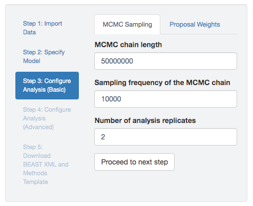
Figure 2.3: MCMC settings. You can specify the simulation length, sampling frequency, and number of replicate simulations.
2.3.3 Proposal Weights
Before discussing proposal weights, it may be helpful to first describe the goal that we are trying to achieve by adjusting proposal weights, and the diagnostics we use to assess our proximity to that goal. As described above, the MCMC simulation length is the total number of MCMC cycles (or generations), the sampling frequency is interval (in number of cycles) at which we write the state of the chain to our log files, such that the number of samples in our log file is the chain length divided by the sampling frequency. Imagine, for example, that we run an MCMC simulation for a length of 1,000,000 cycles with a sampling frequency of 100. We will have sampled 10,000 parameter values, however, the autocorrelation of MCMC states means that we have fewer than 10,000 independent samples.
To estimate the number of effectively independent samples in our log file, we need to compute the Effective Sample Size (ESS) diagnostic. This summary statistic, in turn, relies on a second MCMC summary statistic, the Autocorrelation Time (ACT) diagnostic. The ACT statistic indicates the number of successive MCMC samples over which the values for a given parameter are correlated. Accordingly, the ESS for a given parameter is simply the total number of MCMC samples divided by the ACT for that parameter. For example, imagine that the average dispersal rate parameter, \(\mu\), in our hypothetical MCMC scenario has an autocorrelation time of 100, then the ESS for this parameter is \(10,000 \div 100 = 100\).
The objective is to achieve a sufficiently large ESS value for every (hyper)parameter in our model. The threshold for the minimal ESS value is somewhat arbitrary; by convention, an ESS \(\geq 200\) is considered adequate. [As an aside, it may be useful to augment this arbitrary ESS threshold by visually inspecting the distribution of sampled parameter values. Our objective is to collect an adequate number of samples for a given parameter in order to estimate its marginal posterior probability distribution. Accordingly, if we have collected an adequate number of samples for a given parameter, a histogram of those samples (e.g., plotted in Tracer) should resemble a probability distribution.]
We might be tempted to focus largely/exclusively on the ESS values of the ‘focal’ parameters of our model (while ignoring those for the ‘nuisance’ parameters in our model). However, this would be unwise. Our assignment of a parameter to focal or nuisance status is entirely subjective: we are free to make inferences about (focus on) any parameter in our model by summarizing the samples in the corresponding column of our log file. Nevertheless, the reliability of these marginal posterior probability distributions (based on a column of our log file) depends on an adequate approximation of the corresponding joint posterior probability distribution (all of the columns of our log file). In other words, all of the parameters of our model collectively (jointly) describe the process that gave rise to our observations, so a reliable estimate of any parameter requires that we adequately approximate all model parameters.
Virtually any MCMC simulation—if run long enough—will eventually achieve adequate ESS values for all parameters.
It is common for ESS values to vary substantially across parameters; i.e., where the ESS values for most parameters are extremely large by the time we achieve a minimal ESS value for one or two ‘straggler’ parameters.
The objective is to achieve adequate ESS values for all parameters from the shortest possible MCMC simulation; this requires that the ESS values for all parameters are approximately equal (i.e., such that all parameters reach adequate ESS values at the same point in the MCMC simulation).
We can control the uniformity of the ESS values—and thereby optimize the efficiency of our MCMC simulation—by adjusting the proposal weights.
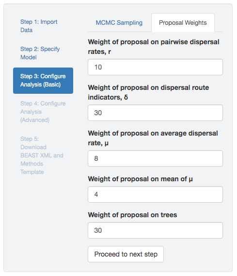
Figure 2.4: Specify proposal weights.
The proposal weights in BEAST are relative.
For example, an MCMC simulation with two proposal mechanisms—\(\alpha\) with proposal weight 1, and \(\beta\) with proposal weight 2—is identical to the setting with proposal weights \(\alpha = 10\) and \(\beta = 20\) (i.e., under both settings, the probability that we propose a change to parameter \(\alpha\) is \(1 \div (1 + 2) = 0.33 \equiv 10 \div (10 + 20) = 0.33\)).
It is common for the ESS values of some parameters to increase more slowly than others.
These difficult parameters have longer autocorrelation times (ACT), owing to low acceptance rates for proposed changes to these parameters and/or because of correlations involving these parameters.
The general idea is to increase the proposal weight for these difficult parameters so that their ESS values increase at approximately the same rate as those of other parameters.
Our experience with a given model and proposal mechanisms may inform our choice of initial proposal weights. (In fact, our experience with discrete discrete-geographic models and proposals informed our choice of default proposal weights specified in PrioriTree, Figure 2.4) However, the optimal proposal weights will vary from analysis to analysis; therefore identifying the optimal set of proposal weights is yet again a trial-and-error process.
We suggest the following iterative procedure for optimizing proposal weights (and MCMC efficiency). First, perform a relatively short, preliminary (‘shakedown’) MCMC simulation using the default PrioriTree proposal weights. Next, examine the resulting ESS values for all of the parameters. If the ESS values are strongly uneven—i.e, where most parameter values have similar ESS values, but one or a few have very low ESS values—increase the proposal weights for the parameters with relatively low ESS values (and/or decrease the proposal weights for the parameters with relatively high ESS values). Iterate this process—run a shakedown MCMC simulation, assess ESS values, and adjust proposal weights—until the ESS values for all parameters are approximately uniform. Then set up your final MCMC simulations using the optimized proposal weights, running each replicate MCMC simulation until the ESS value for each parameter is \(\geq 200\).
A final note about the size of log files. If the length of the MCMC simulation required to achieve adequate ESS values for all parameters results in MCMC log files becoming prohibitively large, you may wish to decrease the sampling frequency.