5 Restructuring Data
Sometimes data may not come organized or formatted in the way we would like. The good thing is there are lots of functions that can be used to restructure data.
5.1 Pivots
A pivot is useful for converting data to wide or long format. pivot_longer() will take multiple columns and turn it into one variable. pivot_wider() takes a column and converts it to multiple different variables. A step-by-step breakdown of pivots can be found in section 12.3 of R for Data Science.
We will practice pivoting in the example below.
5.2 Joins
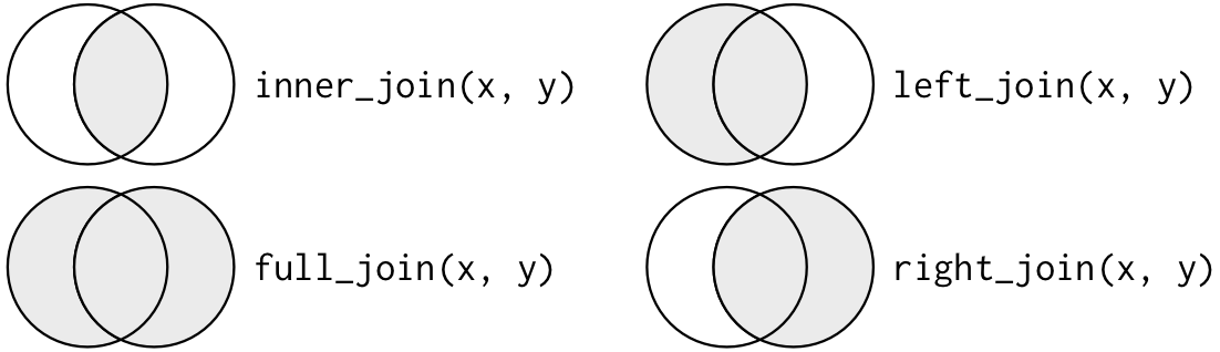
Joins are helpful for combining two separate datasets. They are joined based on the keys, which can be specified by the coder. For now we will refer to the two data frames as x and y. There are four types of joins:
inner_join(): only keeps observations fromxthat have a matching key inyleft_join(): keeps all observations inxright_join(): keeps all observations inyfull_join(): keeps all observations inxandy
Chapter 13 of R for Data Science has a more thorough explanation of joins.
The join functions are part of the dplyr library. This package is in the tidyverse, so it will automatically be loaded if the tidyverse is loaded.
library(dplyr)
set.seed(2023)
5.2.1 Example
We will practice pivoting and joins using the Lahman package.
library(Lahman)Say we want to join the Batting and Fielding tables. Both of them have over 100,000 observations, so let’s filter it down to only look at the 2021 season.
batting21 <- Batting %>%
  filter(yearID == 2021)
batting21 <- battingStats(batting21)

fielding21 <- Fielding %>%
  filter(yearID == 2021)
Let’s take a look at both of these data frames.
batting21| playerID | yearID | stint | teamID | lgID | G | AB | R | H | X2B | X3B | HR | RBI | SB | CS | BB | SO | IBB | HBP | SH | SF | GIDP | BA | PA | TB | SlugPct | OBP | OPS | BABIP |
|---|---|---|---|---|---|---|---|---|---|---|---|---|---|---|---|---|---|---|---|---|---|---|---|---|---|---|---|---|
| swansda01 | 2021 | 1 | ATL | NL | 160 | 588 | 78 | 146 | 33 | 2 | 27 | 88 | 9 | 3 | 52 | 167 | 4 | 5 | 1 | 7 | 7 | 0.248 | 653 | 264 | 0.449 | 0.311 | 0.760 | 0.297 |
| ennsdi01 | 2021 | 1 | TBA | AL | 9 | 0 | 0 | 0 | 0 | 0 | 0 | 0 | 0 | 0 | 0 | 0 | 0 | 0 | 0 | 0 | 0 | NA | 0 | 0 | NA | NA | NA | NA |
| semiema01 | 2021 | 1 | TOR | AL | 162 | 652 | 115 | 173 | 39 | 2 | 45 | 102 | 15 | 1 | 66 | 146 | 0 | 3 | 0 | 3 | 9 | 0.265 | 724 | 351 | 0.538 | 0.334 | 0.872 | 0.276 |
| romanjo03 | 2021 | 1 | TOR | AL | 62 | 0 | 0 | 0 | 0 | 0 | 0 | 0 | 0 | 0 | 0 | 0 | 0 | 0 | 0 | 0 | 0 | NA | 0 | 0 | NA | NA | NA | NA |
| varshda01 | 2021 | 1 | ARI | NL | 95 | 284 | 41 | 70 | 17 | 2 | 11 | 38 | 6 | 0 | 30 | 67 | 3 | 0 | 1 | 0 | 4 | 0.246 | 315 | 124 | 0.437 | 0.318 | 0.755 | 0.286 |
| llovema01 | 2021 | 1 | PHI | NL | 6 | 0 | 0 | 0 | 0 | 0 | 0 | 0 | 0 | 0 | 0 | 0 | 0 | 0 | 0 | 0 | 0 | NA | 0 | 0 | NA | NA | NA | NA |
The data has 29 variables and 1706 observations.
fielding21| playerID | yearID | stint | teamID | lgID | POS | G | GS | InnOuts | PO | A | E | DP | PB | WP | SB | CS | ZR |
|---|---|---|---|---|---|---|---|---|---|---|---|---|---|---|---|---|---|
| penafe01 | 2021 | 1 | LAA | AL | P | 2 | 0 | 5 | 0 | 0 | 0 | 0 | NA | NA | 0 | 0 | NA |
| smithjo05 | 2021 | 2 | SEA | AL | P | 23 | 0 | 54 | 1 | 1 | 0 | 0 | NA | NA | 2 | 0 | NA |
| lintz01 | 2021 | 1 | MIN | AL | OF | 1 | 0 | 6 | 0 | 0 | 0 | 0 | NA | NA | NA | NA | NA |
| valaipa01 | 2021 | 1 | BAL | AL | OF | 3 | 0 | 27 | 3 | 0 | 0 | 0 | NA | NA | NA | NA | NA |
| hildetr01 | 2021 | 1 | NYN | NL | P | 2 | 0 | 7 | 0 | 0 | 0 | 0 | NA | NA | 0 | 0 | NA |
| degotal01 | 2021 | 1 | HOU | AL | 2B | 2 | 2 | 48 | 2 | 0 | 0 | 0 | NA | NA | NA | NA | NA |
The data has 18 variables and 2312 observations.
Before joining these tables, we are going to compute a summarized version of the fielding data and adjust the format.
The pivot_wider() function changes the setup of the data by increasing the number of columns and decreasing the number of rows. This is in the tidyr package, which is part of the tidyverse.
library(tidyr)We will use DJ LeMahieu as an example to help illustrate exactly what pivoting does.
lemahieu <- Fielding %>%
  filter(playerID == "lemahdj01") %>%
arrange(desc(yearID))| playerID | yearID | stint | teamID | lgID | POS | G | GS | InnOuts | PO | A | E | DP | PB | WP | SB | CS | ZR |
|---|---|---|---|---|---|---|---|---|---|---|---|---|---|---|---|---|---|
| lemahdj01 | 2021 | 1 | NYA | AL | 1B | 55 | 33 | 963 | 286 | 13 | 1 | 21 | NA | NA | NA | NA | NA |
| lemahdj01 | 2021 | 1 | NYA | AL | 2B | 83 | 77 | 1989 | 117 | 156 | 2 | 48 | NA | NA | NA | NA | NA |
| lemahdj01 | 2021 | 1 | NYA | AL | 3B | 39 | 36 | 897 | 18 | 62 | 6 | 6 | NA | NA | NA | NA | NA |
| lemahdj01 | 2020 | 1 | NYA | AL | 1B | 11 | 1 | 72 | 24 | 0 | 0 | 1 | NA | NA | NA | NA | NA |
| lemahdj01 | 2020 | 1 | NYA | AL | 2B | 37 | 34 | 812 | 51 | 82 | 4 | 19 | NA | NA | NA | NA | NA |
| lemahdj01 | 2020 | 1 | NYA | AL | 3B | 11 | 11 | 261 | 10 | 16 | 2 | 2 | NA | NA | NA | NA | NA |
| lemahdj01 | 2019 | 1 | NYA | AL | 1B | 40 | 28 | 786 | 215 | 19 | 2 | 24 | NA | NA | NA | NA | NA |
| lemahdj01 | 2019 | 1 | NYA | AL | 2B | 75 | 66 | 1739 | 118 | 155 | 2 | 32 | NA | NA | NA | NA | NA |
| lemahdj01 | 2019 | 1 | NYA | AL | 3B | 52 | 47 | 1200 | 18 | 87 | 4 | 7 | NA | NA | NA | NA | NA |
| lemahdj01 | 2018 | 1 | COL | NL | 2B | 128 | 127 | 3345 | 209 | 378 | 4 | 90 | NA | NA | NA | NA | NA |
| lemahdj01 | 2017 | 1 | COL | NL | 2B | 153 | 151 | 3906 | 251 | 470 | 8 | 106 | NA | NA | NA | NA | NA |
| lemahdj01 | 2016 | 1 | COL | NL | 2B | 146 | 144 | 3728 | 276 | 422 | 6 | 91 | NA | NA | NA | NA | NA |
| lemahdj01 | 2015 | 1 | COL | NL | 2B | 149 | 146 | 3852 | 300 | 452 | 9 | 120 | NA | NA | NA | NA | NA |
| lemahdj01 | 2014 | 1 | COL | NL | 1B | 1 | 0 | 3 | 0 | 0 | 0 | 0 | NA | NA | NA | NA | NA |
| lemahdj01 | 2014 | 1 | COL | NL | 2B | 144 | 135 | 3539 | 257 | 413 | 6 | 99 | NA | NA | NA | NA | NA |
| lemahdj01 | 2014 | 1 | COL | NL | 3B | 7 | 4 | 115 | 2 | 5 | 0 | 0 | NA | NA | NA | NA | NA |
| lemahdj01 | 2014 | 1 | COL | NL | SS | 1 | 0 | 3 | 0 | 0 | 0 | 0 | NA | NA | NA | NA | NA |
| lemahdj01 | 2013 | 1 | COL | NL | 1B | 1 | 0 | 3 | 2 | 0 | 0 | 0 | NA | NA | NA | NA | NA |
| lemahdj01 | 2013 | 1 | COL | NL | 2B | 90 | 86 | 2250 | 168 | 271 | 3 | 57 | NA | NA | NA | NA | NA |
| lemahdj01 | 2013 | 1 | COL | NL | 3B | 14 | 9 | 302 | 6 | 24 | 0 | 2 | NA | NA | NA | NA | NA |
| lemahdj01 | 2013 | 1 | COL | NL | SS | 1 | 0 | 3 | 0 | 0 | 0 | 0 | NA | NA | NA | NA | NA |
| lemahdj01 | 2012 | 1 | COL | NL | 1B | 1 | 0 | 9 | 1 | 0 | 0 | 0 | NA | NA | NA | NA | NA |
| lemahdj01 | 2012 | 1 | COL | NL | 2B | 67 | 60 | 1527 | 105 | 204 | 2 | 33 | NA | NA | NA | NA | NA |
| lemahdj01 | 2012 | 1 | COL | NL | 3B | 9 | 5 | 138 | 2 | 8 | 0 | 0 | NA | NA | NA | NA | NA |
| lemahdj01 | 2012 | 1 | COL | NL | SS | 2 | 0 | 6 | 0 | 0 | 0 | 0 | NA | NA | NA | NA | NA |
| lemahdj01 | 2011 | 1 | CHN | NL | 1B | 1 | 1 | 24 | 8 | 0 | 0 | 1 | NA | NA | NA | NA | NA |
| lemahdj01 | 2011 | 1 | CHN | NL | 2B | 15 | 8 | 233 | 16 | 22 | 0 | 5 | NA | NA | NA | NA | NA |
| lemahdj01 | 2011 | 1 | CHN | NL | 3B | 11 | 6 | 180 | 6 | 12 | 4 | 5 | NA | NA | NA | NA | NA |
Currently the data is set up so if a player plays multiple positions in one season there will be a separate row for each. There are three rows for the 2021 season; one for first base, one for second base, and one for third base. We want to pivot the data so each player only has one row per season, but create columns to show which positions they played.
This is what the data looks like when pivoted:| playerID | yearID | stint | teamID | Inn_1B | Inn_2B | Inn_3B | Inn_SS |
|---|---|---|---|---|---|---|---|
| lemahdj01 | 2021 | 1 | NYA | 963 | 1989 | 897 | 0 |
| lemahdj01 | 2020 | 1 | NYA | 72 | 812 | 261 | 0 |
| lemahdj01 | 2019 | 1 | NYA | 786 | 1739 | 1200 | 0 |
| lemahdj01 | 2018 | 1 | COL | 0 | 3345 | 0 | 0 |
| lemahdj01 | 2017 | 1 | COL | 0 | 3906 | 0 | 0 |
| lemahdj01 | 2016 | 1 | COL | 0 | 3728 | 0 | 0 |
| lemahdj01 | 2015 | 1 | COL | 0 | 3852 | 0 | 0 |
| lemahdj01 | 2014 | 1 | COL | 3 | 3539 | 115 | 3 |
| lemahdj01 | 2013 | 1 | COL | 3 | 2250 | 302 | 3 |
| lemahdj01 | 2012 | 1 | COL | 9 | 1527 | 138 | 6 |
| lemahdj01 | 2011 | 1 | CHN | 24 | 233 | 180 | 0 |
Each position LeMahieu has played at has it’s own column.
Now it’s time to pivot the entire ‘fielding21’ data frame.
names_from specifies which existing column to use for the new column names. In this case it is ‘POS’ - instead of having one column for position, each different position will now have their own column. values_from says what values should be in those new columns. In this example that is ‘InnOuts’ - the data values in the newly created columns are how many outs a player played in said position.
fielding21_wide <- fielding21 %>%
  pivot_wider(names_from = POS, values_from = InnOuts) %>%
  select(playerID:lgID, P:`2B`) %>%
  replace_na(list(C = 0, `1B` = 0, `2B` = 0, `3B` = 0,
                  SS = 0, P = 0, OF = 0)) %>%
  summarize(Inn_1B = sum(`1B`),
            Inn_2B = sum(`2B`),
            Inn_3B = sum(`3B`),
            Inn_SS = sum(SS),
            Inn_C = sum(C),
            Inn_OF = sum(OF),
            Inn_P = sum(P),
.by = c(playerID, yearID, stint, teamID))| playerID | yearID | stint | teamID | Inn_1B | Inn_2B | Inn_3B | Inn_SS | Inn_C | Inn_OF | Inn_P |
|---|---|---|---|---|---|---|---|---|---|---|
| smithjo05 | 2021 | 1 | HOU | 0 | 0 | 0 | 0 | 0 | 0 | 65 |
| bummeaa01 | 2021 | 1 | CHA | 0 | 0 | 0 | 0 | 0 | 0 | 169 |
| altuvjo01 | 2021 | 1 | HOU | 0 | 3789 | 0 | 0 | 0 | 0 | 0 |
| woodhu01 | 2021 | 1 | TEX | 0 | 0 | 0 | 0 | 0 | 0 | 15 |
| dickeco01 | 2021 | 1 | MIA | 0 | 0 | 0 | 0 | 0 | 1275 | 0 |
| perezmi03 | 2021 | 1 | PIT | 3 | 0 | 0 | 0 | 1465 | 0 | 0 |
This data frame has 11 variables and 1697 observations.
Using a similar process we could find a player’s primary position, if that was desired.
fielding21 %>%
  select(playerID:InnOuts) %>%
  group_by(playerID, stint) %>%
  arrange(desc(InnOuts), .by_group = TRUE) %>%
  ungroup() %>%
  mutate(InnProp = InnOuts / sum(InnOuts),
         POS_Q = ifelse(InnProp > 0.25, POS, NA),
         .by = c(playerID, stint)) %>%
  group_by(playerID, stint) %>%
  summarize(Pos = paste(na.omit(POS_Q), collapse = "/")) %>%
  head(20) %>%
  kable() %>%
  kable_styling("striped") %>%
scroll_box(height = "300px")| playerID | stint | Pos |
|---|---|---|
| abadfe01 | 1 | P |
| abbotco01 | 1 | P |
| abreual01 | 1 | P |
| abreubr01 | 1 | P |
| abreujo02 | 1 | 1B |
| acevedo01 | 1 | P |
| acunaro01 | 1 | OF |
| adamewi01 | 1 | SS |
| adamewi01 | 2 | SS |
| adamja01 | 1 | P |
| adamsau02 | 1 | P |
| adamsma01 | 1 | 1B |
| adamsri03 | 1 | C |
| adamsri03 | 2 | C |
| adelljo01 | 1 | OF |
| adonjo01 | 1 | P |
| adriaeh01 | 1 | OF/3B |
| aguilje01 | 1 | 1B |
| aguilmi01 | 1 | P |
| ahmedni01 | 1 | SS |
Now we are ready to practice some joins!
Inner Join
Remember, a key must be present in both datasets to be joined. There are three columns that overlap between the two: ‘playerID’, ‘yearID’, and ‘stint’. We will specify that these variables are the keys in the join_by argument.
join_inner <- inner_join(batting21, fielding21_wide, by = join_by(playerID, yearID, stint))| playerID | yearID | stint | teamID.x | lgID | G | AB | R | H | X2B | X3B | HR | RBI | SB | CS | BB | SO | IBB | HBP | SH | SF | GIDP | BA | PA | TB | SlugPct | OBP | OPS | BABIP | teamID.y | Inn_1B | Inn_2B | Inn_3B | Inn_SS | Inn_C | Inn_OF | Inn_P |
|---|---|---|---|---|---|---|---|---|---|---|---|---|---|---|---|---|---|---|---|---|---|---|---|---|---|---|---|---|---|---|---|---|---|---|---|---|
| topaju01 | 2021 | 1 | MIL | NL | 4 | 1 | 0 | 0 | 0 | 0 | 0 | 0 | 0 | 0 | 0 | 1 | 0 | 0 | 0 | 0 | 0 | 0.000 | 1 | 0 | 0.000 | 0.000 | 0.000 | NaN | MIL | 0 | 0 | 0 | 0 | 0 | 0 | 10 |
| cottojh01 | 2021 | 1 | TEX | AL | 23 | 0 | 0 | 0 | 0 | 0 | 0 | 0 | 0 | 0 | 0 | 0 | 0 | 0 | 0 | 0 | 0 | NA | 0 | 0 | NA | NA | NA | NA | TEX | 0 | 0 | 0 | 0 | 0 | 0 | 92 |
| freelky01 | 2021 | 1 | COL | NL | 25 | 33 | 3 | 6 | 1 | 0 | 0 | 4 | 0 | 0 | 2 | 17 | 0 | 0 | 4 | 1 | 0 | 0.182 | 40 | 7 | 0.212 | 0.222 | 0.434 | 0.353 | COL | 0 | 0 | 0 | 0 | 0 | 3 | 362 |
| fostema01 | 2021 | 1 | CHA | AL | 37 | 0 | 0 | 0 | 0 | 0 | 0 | 0 | 0 | 0 | 0 | 0 | 0 | 0 | 0 | 0 | 0 | NA | 0 | 0 | NA | NA | NA | NA | CHA | 0 | 0 | 0 | 0 | 0 | 0 | 117 |
| detmere01 | 2021 | 1 | LAA | AL | 5 | 1 | 0 | 0 | 0 | 0 | 0 | 0 | 0 | 0 | 1 | 1 | 0 | 0 | 0 | 0 | 0 | 0.000 | 2 | 0 | 0.000 | 0.500 | 0.500 | NaN | LAA | 0 | 0 | 0 | 0 | 0 | 0 | 62 |
| smeltde01 | 2021 | 1 | MIN | AL | 1 | 0 | 0 | 0 | 0 | 0 | 0 | 0 | 0 | 0 | 0 | 0 | 0 | 0 | 0 | 0 | 0 | NA | 0 | 0 | NA | NA | NA | NA | MIN | 0 | 0 | 0 | 0 | 0 | 0 | 14 |
This creates a new data frame with 37 variables and 1697 observations. It is the same amount of rows as fielding21_wide, the smaller dataset.
Left Join
The code for each type of join is identical, besides the first word of the join function.
join_left <- left_join(batting21, fielding21_wide, by = join_by(playerID, yearID, stint))| playerID | yearID | stint | teamID.x | lgID | G | AB | R | H | X2B | X3B | HR | RBI | SB | CS | BB | SO | IBB | HBP | SH | SF | GIDP | BA | PA | TB | SlugPct | OBP | OPS | BABIP | teamID.y | Inn_1B | Inn_2B | Inn_3B | Inn_SS | Inn_C | Inn_OF | Inn_P |
|---|---|---|---|---|---|---|---|---|---|---|---|---|---|---|---|---|---|---|---|---|---|---|---|---|---|---|---|---|---|---|---|---|---|---|---|---|
| pivetni01 | 2021 | 1 | BOS | AL | 31 | 2 | 0 | 0 | 0 | 0 | 0 | 0 | 0 | 0 | 0 | 2 | 0 | 0 | 0 | 0 | 0 | 0.000 | 2 | 0 | 0.000 | 0.000 | 0.000 | NaN | BOS | 0 | 0 | 0 | 0 | 0 | 0 | 465 |
| leekh01 | 2021 | 1 | NYN | NL | 11 | 18 | 2 | 1 | 1 | 0 | 0 | 1 | 0 | 0 | 0 | 13 | 0 | 0 | 0 | 0 | 0 | 0.056 | 18 | 2 | 0.111 | 0.056 | 0.167 | 0.200 | NYN | 0 | 0 | 0 | 0 | 0 | 134 | 0 |
| bonifjo01 | 2021 | 1 | PHI | NL | 7 | 11 | 0 | 1 | 0 | 0 | 0 | 2 | 0 | 0 | 1 | 6 | 0 | 0 | 0 | 0 | 0 | 0.091 | 12 | 1 | 0.091 | 0.167 | 0.258 | 0.200 | PHI | 0 | 0 | 0 | 0 | 0 | 63 | 0 |
| carraca01 | 2021 | 1 | NYN | NL | 12 | 15 | 0 | 0 | 0 | 0 | 0 | 0 | 0 | 0 | 0 | 10 | 0 | 0 | 4 | 0 | 0 | 0.000 | 19 | 0 | 0.000 | 0.000 | 0.000 | 0.000 | NYN | 0 | 0 | 0 | 0 | 0 | 0 | 161 |
| minayju01 | 2021 | 1 | MIN | AL | 29 | 0 | 0 | 0 | 0 | 0 | 0 | 0 | 0 | 0 | 0 | 0 | 0 | 0 | 0 | 0 | 0 | NA | 0 | 0 | NA | NA | NA | NA | MIN | 0 | 0 | 0 | 0 | 0 | 0 | 120 |
| kirkal01 | 2021 | 1 | TOR | AL | 60 | 165 | 19 | 40 | 8 | 0 | 8 | 24 | 0 | 0 | 19 | 22 | 0 | 3 | 0 | 2 | 7 | 0.242 | 189 | 72 | 0.436 | 0.328 | 0.764 | 0.234 | TOR | 0 | 0 | 0 | 0 | 1014 | 0 | 0 |
This creates a new data frame with 37 variables and 37 observations. It is the same amount of rows as batting21, the left dataset.
Right Join
join_right <- right_join(batting21, fielding21_wide, by = join_by(playerID, yearID, stint))| playerID | yearID | stint | teamID.x | lgID | G | AB | R | H | X2B | X3B | HR | RBI | SB | CS | BB | SO | IBB | HBP | SH | SF | GIDP | BA | PA | TB | SlugPct | OBP | OPS | BABIP | teamID.y | Inn_1B | Inn_2B | Inn_3B | Inn_SS | Inn_C | Inn_OF | Inn_P |
|---|---|---|---|---|---|---|---|---|---|---|---|---|---|---|---|---|---|---|---|---|---|---|---|---|---|---|---|---|---|---|---|---|---|---|---|---|
| guerrja01 | 2021 | 1 | WAS | NL | 6 | 1 | 0 | 0 | 0 | 0 | 0 | 0 | 0 | 0 | 0 | 1 | 0 | 0 | 0 | 0 | 0 | 0.000 | 1 | 0 | 0.0 | 0.000 | 0.000 | NaN | WAS | 0 | 0 | 0 | 0 | 0 | 0 | 18 |
| newsolj01 | 2021 | 1 | SEA | AL | 7 | 0 | 0 | 0 | 0 | 0 | 0 | 0 | 0 | 0 | 0 | 0 | 0 | 0 | 0 | 0 | 0 | NA | 0 | 0 | NA | NA | NA | NA | SEA | 0 | 0 | 0 | 0 | 0 | 0 | 44 |
| lowthza01 | 2021 | 1 | BAL | AL | 10 | 0 | 0 | 0 | 0 | 0 | 0 | 0 | 0 | 0 | 0 | 0 | 0 | 0 | 0 | 0 | 0 | NA | 0 | 0 | NA | NA | NA | NA | BAL | 0 | 0 | 0 | 0 | 0 | 0 | 89 |
| ruizri01 | 2021 | 2 | COL | NL | 30 | 35 | 1 | 6 | 1 | 0 | 0 | 4 | 0 | 0 | 3 | 9 | 0 | 0 | 0 | 2 | 0 | 0.171 | 40 | 7 | 0.2 | 0.225 | 0.425 | 0.214 | COL | 24 | 0 | 75 | 0 | 0 | 9 | 0 |
| brachbr01 | 2021 | 1 | CIN | NL | 35 | 0 | 0 | 0 | 0 | 0 | 0 | 0 | 0 | 0 | 0 | 0 | 0 | 0 | 0 | 0 | 0 | NA | 0 | 0 | NA | NA | NA | NA | CIN | 0 | 0 | 0 | 0 | 0 | 0 | 90 |
| garzara01 | 2021 | 2 | MIN | AL | 18 | 0 | 0 | 0 | 0 | 0 | 0 | 0 | 0 | 0 | 0 | 0 | 0 | 0 | 0 | 0 | 0 | NA | 0 | 0 | NA | NA | NA | NA | MIN | 0 | 0 | 0 | 0 | 0 | 0 | 58 |
This creates a new data frame with 37 variables and 37 observations. It is the same amount of rows as fielding21_wide, the right dataset.
Full Join
join_full <- full_join(batting21, fielding21_wide, by = join_by(playerID, yearID, stint))| playerID | yearID | stint | teamID.x | lgID | G | AB | R | H | X2B | X3B | HR | RBI | SB | CS | BB | SO | IBB | HBP | SH | SF | GIDP | BA | PA | TB | SlugPct | OBP | OPS | BABIP | teamID.y | Inn_1B | Inn_2B | Inn_3B | Inn_SS | Inn_C | Inn_OF | Inn_P |
|---|---|---|---|---|---|---|---|---|---|---|---|---|---|---|---|---|---|---|---|---|---|---|---|---|---|---|---|---|---|---|---|---|---|---|---|---|
| minormi01 | 2021 | 1 | KCA | AL | 28 | 7 | 0 | 0 | 0 | 0 | 0 | 0 | 0 | 0 | 0 | 4 | 0 | 0 | 0 | 0 | 0 | 0.000 | 7 | 0 | 0.000 | 0.000 | 0.000 | 0.000 | KCA | 0 | 0 | 0 | 0 | 0 | 0 | 476 |
| urquijo01 | 2021 | 1 | HOU | AL | 20 | 4 | 0 | 1 | 0 | 0 | 0 | 0 | 0 | 0 | 0 | 3 | 0 | 0 | 0 | 0 | 0 | 0.250 | 4 | 1 | 0.250 | 0.250 | 0.500 | 1.000 | HOU | 0 | 0 | 0 | 0 | 0 | 0 | 321 |
| antonte01 | 2021 | 1 | CIN | NL | 23 | 3 | 1 | 0 | 0 | 0 | 0 | 0 | 0 | 0 | 1 | 3 | 0 | 0 | 1 | 0 | 0 | 0.000 | 5 | 0 | 0.000 | 0.250 | 0.250 | NaN | CIN | 0 | 0 | 0 | 0 | 0 | 0 | 101 |
| holadbr01 | 2021 | 1 | ARI | NL | 13 | 31 | 2 | 6 | 2 | 0 | 0 | 1 | 0 | 0 | 1 | 15 | 0 | 2 | 0 | 0 | 0 | 0.194 | 34 | 8 | 0.258 | 0.265 | 0.523 | 0.375 | ARI | 0 | 0 | 0 | 0 | 255 | 0 | 3 |
| mccanja02 | 2021 | 1 | NYN | NL | 121 | 375 | 29 | 87 | 12 | 1 | 10 | 46 | 1 | 2 | 32 | 115 | 1 | 2 | 0 | 3 | 12 | 0.232 | 412 | 131 | 0.349 | 0.294 | 0.643 | 0.304 | NYN | 135 | 0 | 0 | 0 | 2479 | 0 | 0 |
| bruihju01 | 2021 | 1 | LAN | NL | 21 | 0 | 0 | 0 | 0 | 0 | 0 | 0 | 0 | 0 | 1 | 0 | 0 | 0 | 0 | 0 | 0 | NA | 1 | 0 | NA | 1.000 | NA | NA | LAN | 0 | 0 | 0 | 0 | 0 | 0 | 56 |
This creates a new data frame with 37 variables and 37 observations. It is the same amount of rows as as batting21, the larger dataset.
5.2.2 Another Example
Let’s try another example. This time we will use the Pitching and Salaries tables. First we will filter both down to one season (2016).
pitching16 <- Pitching %>%
  filter(yearID == 2016)

salaries16 <- Salaries %>%
filter(yearID == 2016)| playerID | yearID | stint | teamID | lgID | W | L | G | GS | CG | SHO | SV | IPouts | H | ER | HR | BB | SO | BAOpp | ERA | IBB | WP | HBP | BK | BFP | GF | R | SH | SF | GIDP |
|---|---|---|---|---|---|---|---|---|---|---|---|---|---|---|---|---|---|---|---|---|---|---|---|---|---|---|---|---|---|
| mccarbr01 | 2016 | 1 | LAN | NL | 2 | 3 | 10 | 9 | 0 | 0 | 0 | 120 | 29 | 22 | 2 | 26 | 44 | 0.207 | 4.95 | 1 | 2 | 2 | 0 | 171 | 0 | 24 | 1 | 2 | 3 |
| wimmeal01 | 2016 | 1 | MIN | AL | 1 | 3 | 16 | 0 | 0 | 0 | 0 | 52 | 14 | 8 | 2 | 11 | 14 | 0.237 | 4.15 | 1 | 0 | 0 | 0 | 72 | 2 | 8 | 0 | 2 | 3 |
| osullse01 | 2016 | 1 | BOS | AL | 2 | 0 | 5 | 4 | 0 | 0 | 0 | 64 | 30 | 16 | 3 | 6 | 13 | 0.337 | 6.75 | 0 | 2 | 2 | 0 | 98 | 1 | 17 | 0 | 1 | 1 |
| zastrro01 | 2016 | 1 | CHN | NL | 1 | 0 | 8 | 1 | 0 | 0 | 0 | 48 | 12 | 2 | 0 | 5 | 17 | 0.207 | 1.13 | 0 | 0 | 1 | 0 | 66 | 1 | 3 | 0 | 2 | 1 |
| salasfe01 | 2016 | 2 | NYN | NL | 0 | 1 | 17 | 0 | 0 | 0 | 0 | 52 | 11 | 4 | 3 | 0 | 19 | 0.177 | 2.08 | 0 | 1 | 0 | 0 | 62 | 2 | 4 | 0 | 0 | 1 |
| boydma01 | 2016 | 1 | DET | AL | 6 | 5 | 20 | 18 | 0 | 0 | 0 | 292 | 97 | 49 | 17 | 29 | 82 | 0.258 | 4.53 | 0 | 1 | 4 | 0 | 412 | 1 | 51 | 0 | 3 | 8 |
The data has 30 variables and 824 observations.
salaries16| yearID | teamID | lgID | playerID | salary |
|---|---|---|---|---|
| 2016 | SEA | AL | lindad01 | 8000000 |
| 2016 | OAK | AL | fuldsa01 | 1925000 |
| 2016 | MIA | NL | jacksed01 | 507500 |
| 2016 | LAA | AL | smithjo05 | 5250000 |
| 2016 | BOS | AL | vazquch01 | 513000 |
| 2016 | CIN | NL | cothaca01 | 509675 |
The data has 5 variables and 853 observations.
The common columns are ‘playerID’, ‘yearID’, and ‘teamID’, and ‘leagueID’. Let’s see what happens if we do not use all four of these variables as keys while joining.
join_half_keys <- inner_join(pitching16, salaries16, join_by(playerID, yearID))| playerID | yearID | stint | teamID.x | lgID.x | W | L | G | GS | CG | SHO | SV | IPouts | H | ER | HR | BB | SO | BAOpp | ERA | IBB | WP | HBP | BK | BFP | GF | R | SH | SF | GIDP | teamID.y | lgID.y | salary |
|---|---|---|---|---|---|---|---|---|---|---|---|---|---|---|---|---|---|---|---|---|---|---|---|---|---|---|---|---|---|---|---|---|
| lobstky01 | 2016 | 1 | PIT | NL | 2 | 0 | 14 | 0 | 0 | 0 | 0 | 75 | 25 | 11 | 2 | 12 | 15 | 0.263 | 3.96 | 1 | 2 | 2 | 0 | 110 | 3 | 11 | 1 | 0 | 4 | PIT | NL | 520000 |
| gonzagi01 | 2016 | 1 | WAS | NL | 11 | 11 | 32 | 32 | 0 | 0 | 0 | 532 | 179 | 90 | 19 | 59 | 171 | 0.262 | 4.57 | 2 | 7 | 9 | 0 | 765 | 0 | 98 | 8 | 5 | 17 | WAS | NL | 12100000 |
| harriwi02 | 2016 | 1 | HOU | AL | 1 | 2 | 66 | 0 | 0 | 0 | 12 | 192 | 52 | 16 | 3 | 15 | 69 | 0.220 | 2.25 | 1 | 4 | 1 | 0 | 255 | 19 | 17 | 1 | 2 | 6 | HOU | AL | 525500 |
| thornma01 | 2016 | 1 | SDN | NL | 1 | 0 | 18 | 0 | 0 | 0 | 0 | 51 | 22 | 11 | 2 | 6 | 9 | 0.314 | 5.82 | 0 | 0 | 1 | 0 | 77 | 8 | 12 | 0 | 0 | 4 | SDN | NL | 1600000 |
| tonkimi01 | 2016 | 1 | MIN | AL | 3 | 2 | 65 | 0 | 0 | 0 | 0 | 215 | 80 | 40 | 13 | 24 | 80 | 0.280 | 5.02 | 0 | 5 | 3 | 0 | 315 | 23 | 46 | 2 | 0 | 7 | MIN | AL | 515000 |
| lestejo01 | 2016 | 1 | CHN | NL | 19 | 5 | 32 | 32 | 2 | 0 | 0 | 608 | 154 | 55 | 21 | 52 | 197 | 0.211 | 2.44 | 0 | 4 | 6 | 0 | 796 | 0 | 57 | 4 | 4 | 15 | CHN | NL | 25000000 |
There are two columns for ‘teamID’ and two columns for ‘lgID’.
Now let’s look at what happens if we use all four common variables as keys.
join_all_keys <- inner_join(pitching16, salaries16, join_by(playerID, yearID, teamID, lgID))| playerID | yearID | stint | teamID | lgID | W | L | G | GS | CG | SHO | SV | IPouts | H | ER | HR | BB | SO | BAOpp | ERA | IBB | WP | HBP | BK | BFP | GF | R | SH | SF | GIDP | salary |
|---|---|---|---|---|---|---|---|---|---|---|---|---|---|---|---|---|---|---|---|---|---|---|---|---|---|---|---|---|---|---|
| morribr01 | 2016 | 1 | MIA | NL | 0 | 0 | 24 | 0 | 0 | 0 | 1 | 53 | 15 | 6 | 4 | 10 | 13 | 0.238 | 3.06 | 1 | 0 | 1 | 0 | 74 | 4 | 7 | 0 | 0 | 2 | 1350000 |
| matusbr01 | 2016 | 1 | BAL | AL | 0 | 0 | 7 | 0 | 0 | 0 | 0 | 18 | 11 | 8 | 3 | 7 | 1 | 0.407 | 12.00 | 0 | 0 | 0 | 0 | 35 | 2 | 8 | 0 | 1 | 1 | 3900000 |
| santihe01 | 2016 | 1 | LAA | AL | 10 | 4 | 22 | 22 | 0 | 0 | 0 | 362 | 104 | 57 | 20 | 57 | 107 | 0.233 | 4.25 | 0 | 2 | 4 | 1 | 515 | 0 | 61 | 3 | 4 | 9 | 5000000 |
| wislema01 | 2016 | 1 | ATL | NL | 7 | 13 | 27 | 26 | 0 | 0 | 1 | 470 | 159 | 87 | 26 | 49 | 115 | 0.259 | 5.00 | 3 | 5 | 4 | 1 | 671 | 1 | 90 | 2 | 3 | 12 | 507500 |
| floydga01 | 2016 | 1 | TOR | AL | 2 | 4 | 28 | 0 | 0 | 0 | 0 | 93 | 23 | 14 | 4 | 8 | 30 | 0.205 | 4.06 | 1 | 4 | 3 | 0 | 124 | 10 | 14 | 0 | 1 | 2 | 1000000 |
| sanchaa01 | 2016 | 1 | TOR | AL | 15 | 2 | 30 | 30 | 0 | 0 | 0 | 576 | 161 | 64 | 15 | 63 | 161 | 0.224 | 3.00 | 0 | 5 | 5 | 0 | 790 | 0 | 69 | 1 | 2 | 14 | 517800 |
There are no repeat columns! Whenever the data frames you want to join share columns, make sure to specify all of them in the join_by argument.
Here’s a graph created from the joined data.
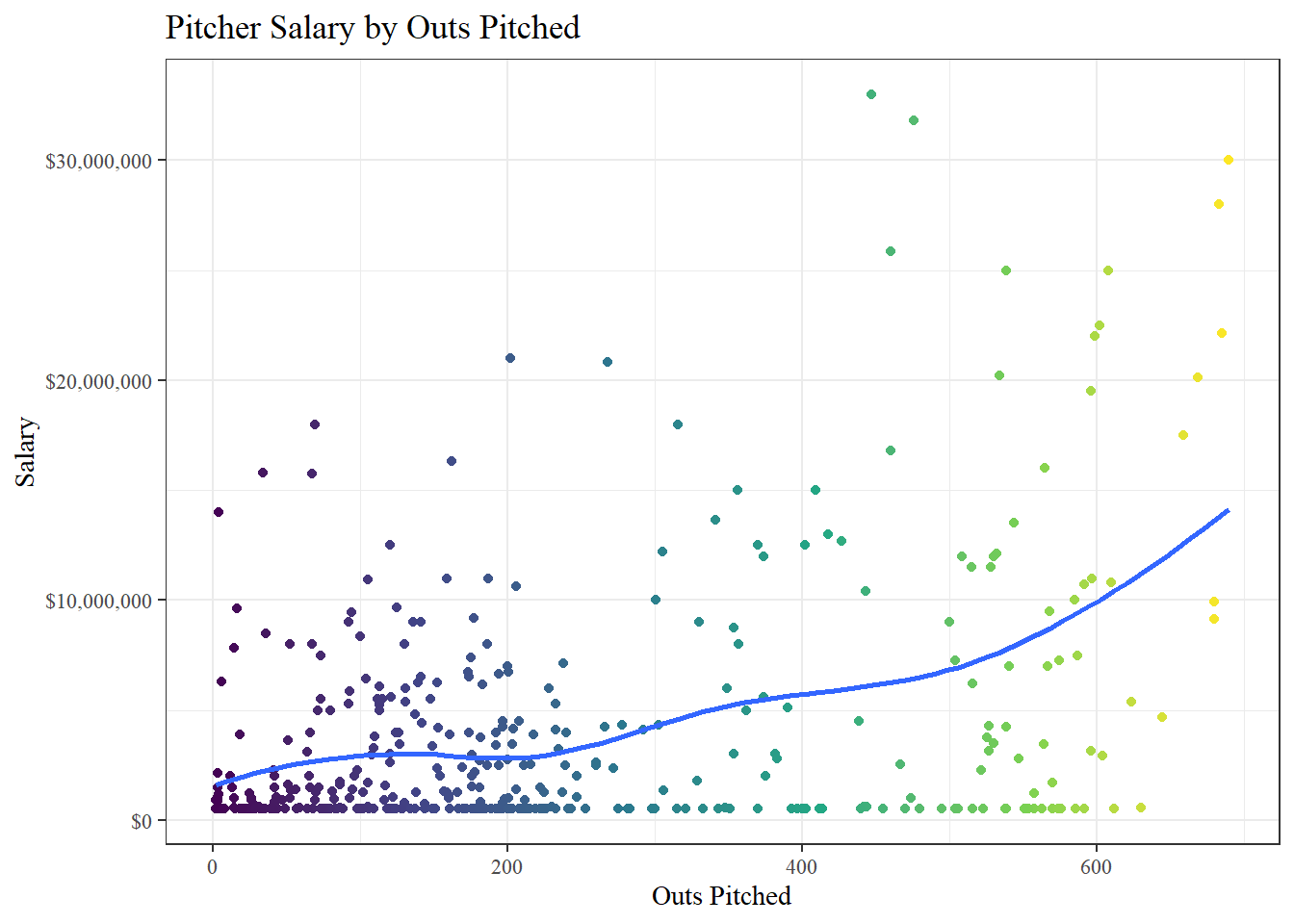
It should be noted that not all players have salary data. This may be because of a variety of reasons such as arbitration, lack of games played, or simply that their salary data is not available.