3 FanGraphs

type of data available: game-by-game, summary statistics (split by Batting, Pitching, and Fielding)

There are two ways to use data from FanGraphs in R:

1. Downloading the data directly from https://www.fangraphs.com/ and importing it into R
2. Using the baseballr package

3.1 FanGraphs Website

The ‘Leaders’ and ‘Teams’ pages will both bring up a dashboard that can easily be downloaded. The data is very customizable. There are several tabs that will show different sets of data. And at the bottom of the page there is an option to select which variables to include in order to make a fully custom report. In the top right corner of the table it says “Export Data”. The data will download as a CSV file.

The file I chose to download is the 2022 Team Batting Stats. If the working directory is set as the source file location, you can use the read_csv() function (from the readr package) with just the file name in quotes. To check the working directory run the function getwd. To change the working directory go to the “Session” menu and select “Set Working Directory”.

fg_download <- read_csv("data/fg_batting.csv")
fg_download <- as.data.frame(fg_download)

Team	G	PA	HR	R	RBI	SB	BB%	K%	ISO	BABIP	AVG	OBP	SLG	wOBA	xwOBA	wRC+	BsR	Off	Def	WAR	Team.
LAD	2326	6247	212	847	812	98	9.7%	22.0%	0.185	0.302	0.257	0.333	0.442	0.337	NA	119	19.9	159.0	1.5	38.9	LAD
NYY	2342	6172	254	807	764	102	10.0%	22.5%	0.185	0.276	0.241	0.325	0.426	0.327	NA	115	-5.7	98.6	39.6	35.1	NYY
STL	2355	6165	197	772	739	95	8.7%	19.9%	0.168	0.289	0.252	0.325	0.420	0.326	NA	114	4.7	102.5	2.8	32.8	STL
NYM	2340	6176	171	772	735	62	8.3%	19.7%	0.153	0.302	0.259	0.332	0.412	0.326	NA	116	-10.7	103.4	-13.0	31.3	NYM
TOR	2445	6158	200	775	756	67	8.1%	20.2%	0.168	0.305	0.264	0.329	0.431	0.331	NA	117	-10.5	110.8	-9.9	31.2	TOR
HOU	2279	6054	214	737	715	83	8.7%	19.5%	0.176	0.278	0.248	0.319	0.424	0.324	NA	112	-8.9	75.0	13.4	29.5	HOU
ATL	2259	6082	243	789	753	87	7.7%	24.6%	0.190	0.303	0.253	0.317	0.443	0.330	NA	111	9.7	85.1	-14.7	28.9	ATL
MIL	2363	6122	219	725	703	96	9.4%	23.9%	0.174	0.279	0.235	0.315	0.409	0.317	NA	104	5.6	30.6	-4.8	24.3	MIL
SEA	2383	6117	197	690	663	83	9.7%	22.8%	0.160	0.272	0.230	0.315	0.390	0.310	NA	107	-10.0	37.5	-14.3	22.9	SEA
CLE	2338	6163	127	698	662	119	7.3%	18.2%	0.129	0.294	0.254	0.316	0.383	0.306	NA	99	13.2	3.8	6.2	21.7	CLE
PHI	2327	6077	205	747	719	105	7.9%	22.4%	0.169	0.299	0.253	0.317	0.422	0.322	NA	106	9.9	50.9	-50.0	21.6	PHI
SDP	2323	6175	153	705	682	49	9.3%	21.5%	0.141	0.289	0.241	0.318	0.382	0.308	NA	102	3.9	16.8	-22.8	21.2	SDP
MIN	2422	6113	178	696	668	38	8.5%	22.1%	0.153	0.295	0.248	0.317	0.401	0.315	NA	107	-20.7	25.1	-19.0	21.1	MIN
TBR	2403	6008	139	666	634	95	8.3%	23.2%	0.138	0.295	0.239	0.309	0.377	0.302	NA	101	4.0	12.9	-15.3	19.8	TBR
ARI	2407	6027	173	702	658	104	8.8%	22.2%	0.155	0.272	0.230	0.304	0.385	0.303	NA	92	25.4	-27.4	13.0	19.8	ARI
BAL	2359	6049	171	674	639	95	7.9%	23.0%	0.154	0.284	0.236	0.305	0.390	0.305	NA	99	12.0	2.7	-15.0	18.9	BAL
TEX	2365	6029	198	707	670	128	7.6%	24.0%	0.157	0.287	0.239	0.301	0.395	0.305	NA	98	18.8	5.0	-16.7	18.9	TEX
BOS	2379	6144	155	735	704	52	7.8%	22.3%	0.152	0.313	0.258	0.321	0.409	0.319	NA	102	-11.5	3.8	-28.4	18.0	BOS
CHC	2388	6072	159	657	620	111	8.3%	23.8%	0.148	0.294	0.238	0.311	0.387	0.307	NA	98	-1.7	-19.4	-35.6	15.7	CHC
SFG	2552	6117	183	716	683	64	9.3%	23.9%	0.156	0.284	0.234	0.315	0.390	0.311	NA	101	3.0	12.6	-69.6	15.6	SFG
CHW	2371	6123	149	686	654	58	6.3%	20.7%	0.131	0.304	0.256	0.310	0.387	0.306	NA	99	-3.0	-12.6	-36.9	15.3	CHW
LAA	2327	5977	190	623	600	77	7.5%	25.7%	0.157	0.289	0.233	0.297	0.390	0.300	NA	93	-0.8	-47.4	-29.4	11.9	LAA
KCR	2372	6010	138	640	613	104	7.7%	21.4%	0.136	0.293	0.244	0.306	0.380	0.302	NA	93	2.2	-48.6	-40.7	10.7	KCR
MIA	2384	5949	144	586	554	122	7.3%	24.0%	0.133	0.284	0.230	0.294	0.363	0.290	NA	88	-2.6	-84.2	-14.8	10.6	MIA
OAK	2394	5863	137	568	537	78	7.4%	23.7%	0.130	0.264	0.216	0.281	0.346	0.277	NA	84	1.4	-105.0	-16.7	6.8	OAK
COL	2265	6105	149	698	669	45	7.4%	21.8%	0.144	0.307	0.254	0.315	0.398	0.312	NA	86	-2.6	-101.9	-38.8	6.8	COL
PIT	2340	5912	158	591	555	89	8.1%	25.3%	0.141	0.277	0.222	0.291	0.364	0.289	NA	84	6.7	-101.8	-32.9	6.7	PIT
WSN	2347	5998	136	603	579	75	7.4%	20.4%	0.129	0.295	0.249	0.310	0.377	0.303	NA	93	-25.1	-75.3	-68.3	6.1	WSN
CIN	2406	5978	156	648	618	58	7.6%	23.9%	0.137	0.290	0.235	0.304	0.372	0.299	NA	84	-15.6	-123.6	-28.4	5.2	CIN
DET	2350	5870	110	557	530	47	6.5%	24.1%	0.115	0.290	0.231	0.286	0.346	0.279	NA	81	-8.6	-133.1	-29.8	2.5	DET

There are a few important things to note about the data. The variables representing walk rate and strikeout rate have ‘%’ in the column name and in the data values. This is not ideal. Those column names must be placed in backticks whenever referenced because of the special character. Another option is to change the name using a function like rename(). To fix the data values use the function str_remove() inside of mutate(). We can simultaneously convert the variables to numeric instead of character with as.numeric().

# renaming the columns
fg_update <- fg_download %>% rename(BB_rate = `BB%`, K_rate = `K%`)

# fixing the data values
fg_update <- fg_update %>% 
  mutate(BB_rate = as.numeric(str_remove(BB_rate, "%")), 
         K_rate = as.numeric(str_remove(K_rate, "%")))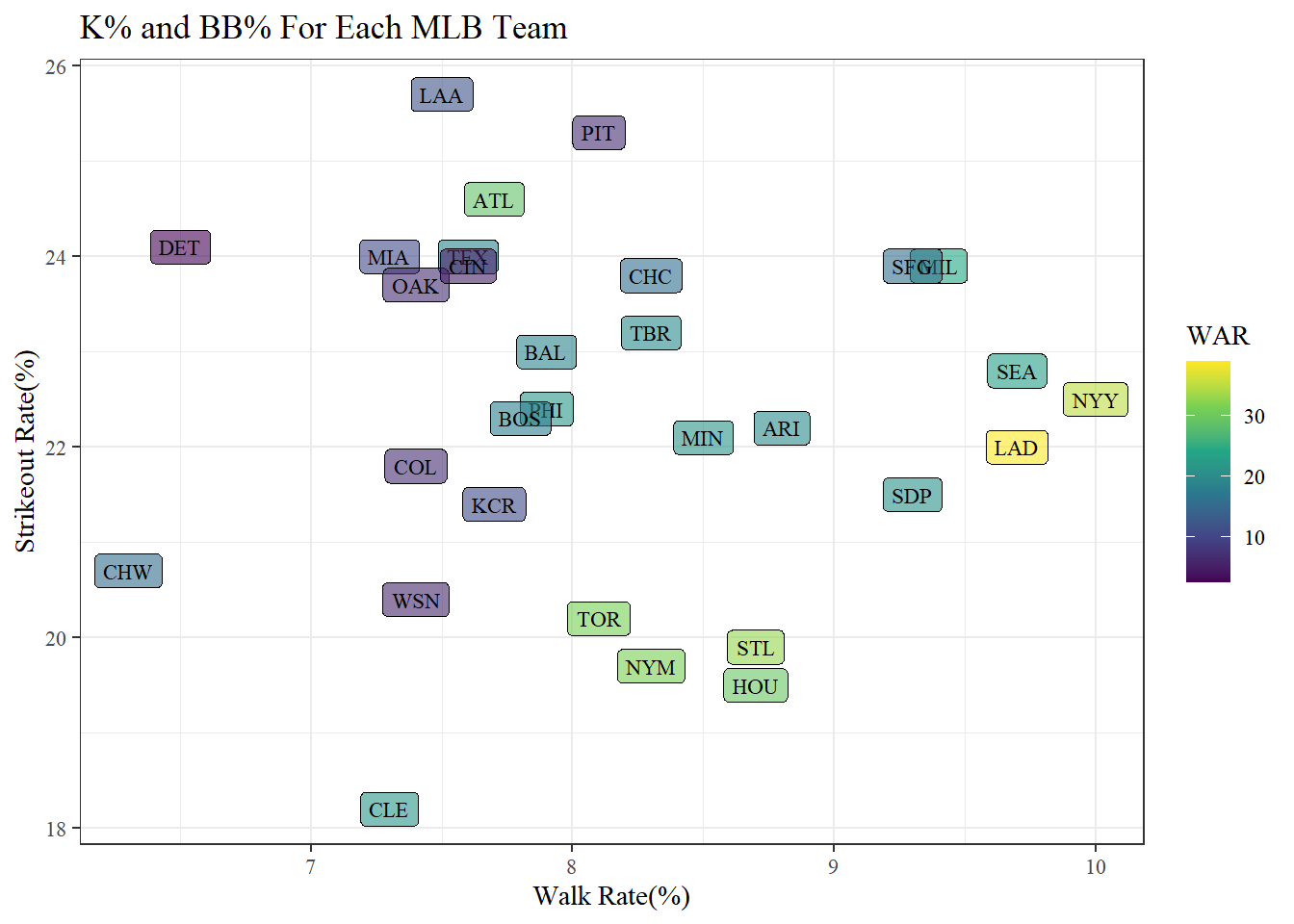

Following the same process as before, I got the 2022 Pitching Leaders. Without changing any settings on FanGraphs, the data frame downloaded has 22 variables and 45 observations.

fg_pitch_leaders <- read_csv("data/fg_pitch_leaders.csv")

Name	Team	W	L	SV	G	GS	IP	K/9	BB/9	HR/9	BABIP	LOB%	GB%	HR/FB	vFA (pi)	ERA	xERA	FIP	xFIP	WAR	playerid
Aaron Nola	PHI	11	13	0	32	32	205.0	10.32	1.27	0.83	0.289	73.0%	43.6%	9.8%	92.9	3.25	2.74	2.58	2.77	6.3	16149
Carlos Rodon	SFG	14	8	0	31	31	178.0	11.98	2.63	0.61	0.293	75.1%	34.1%	6.5%	95.5	2.88	2.64	2.25	2.91	6.2	16137
Justin Verlander	HOU	18	4	0	28	28	175.0	9.51	1.49	0.62	0.240	80.5%	37.9%	6.2%	95.1	1.75	2.66	2.49	3.23	6.1	8700
Sandy Alcantara	MIA	14	9	0	32	32	228.2	8.15	1.97	0.63	0.262	78.8%	53.4%	8.5%	98.0	2.28	2.92	2.99	3.29	5.7	18684
Kevin Gausman	TOR	12	10	0	31	31	174.2	10.56	1.44	0.77	0.363	74.0%	39.2%	8.5%	94.9	3.35	3.34	2.38	2.75	5.7	14107
Shohei Ohtani	LAA	15	9	0	28	28	166.0	11.87	2.39	0.76	0.289	83.1%	41.9%	9.3%	97.4	2.33	2.68	2.40	2.65	5.6	19755
Max Fried	ATL	14	7	0	30	30	185.1	8.26	1.55	0.58	0.280	78.2%	51.2%	7.8%	94.0	2.48	2.85	2.70	3.09	5.0	13743
Shane Bieber	CLE	13	8	0	31	31	200.0	8.91	1.62	0.81	0.287	75.8%	48.2%	10.4%	91.5	2.88	3.51	2.87	2.98	4.9	19427
Corbin Burnes	MIL	12	8	0	33	33	202.0	10.83	2.27	1.02	0.259	76.8%	47.0%	14.1%	96.2	2.94	3.05	3.14	2.85	4.6	19361
Framber Valdez	HOU	17	6	0	31	31	201.1	8.67	3.00	0.49	0.285	75.7%	66.5%	12.5%	94.0	2.82	3.31	3.06	2.99	4.4	17295
Dylan Cease	CHW	14	8	0	32	32	184.0	11.10	3.82	0.78	0.260	82.3%	38.8%	8.4%	96.9	2.20	2.70	3.10	3.50	4.4	18525
Zac Gallen	ARI	12	4	0	31	31	184.0	9.39	2.30	0.73	0.237	78.0%	46.0%	9.1%	93.9	2.54	3.17	3.05	3.31	4.3	19291
Yu Darvish	SDP	16	8	0	30	30	194.2	9.11	1.71	1.02	0.250	78.2%	36.9%	9.6%	95.0	3.10	3.49	3.31	3.58	4.2	13074
Logan Webb	SFG	15	9	0	32	32	192.1	7.63	2.29	0.51	0.293	71.8%	56.7%	8.3%	92.4	2.90	3.59	3.03	3.31	4.2	17995
Alek Manoah	TOR	16	7	0	31	31	196.2	8.24	2.33	0.73	0.244	82.6%	37.5%	7.1%	93.9	2.24	3.31	3.35	3.97	4.1	26410
Tyler Anderson	LAD	15	5	0	30	28	178.2	6.95	1.71	0.71	0.256	77.8%	40.1%	6.4%	90.7	2.57	3.10	3.31	4.10	4.0	12880
Jose Quintana		6	7	0	32	32	165.2	7.44	2.55	0.43	0.302	74.2%	46.4%	5.3%	91.3	2.93	3.86	2.99	3.72	4.0	11423
Martin Perez	TEX	12	8	0	32	32	196.1	7.75	3.16	0.50	0.295	77.0%	51.4%	6.5%	92.9	2.89	3.59	3.27	3.80	3.8	6902
Triston McKenzie	CLE	11	11	0	31	30	191.1	8.94	2.07	1.18	0.237	80.3%	32.7%	10.3%	92.7	2.96	3.54	3.59	3.77	3.6	18000
Shane McClanahan	TBR	12	8	0	28	28	166.1	10.50	2.06	1.03	0.251	80.5%	50.2%	15.7%	97.0	2.54	2.79	3.00	2.60	3.5	21483
Joe Musgrove	SDP	10	7	0	30	30	181.0	9.15	2.09	1.09	0.276	79.8%	44.6%	12.3%	92.9	2.93	3.27	3.59	3.47	3.5	12970
Merrill Kelly	ARI	13	8	0	33	33	200.1	7.95	2.74	0.94	0.269	76.3%	42.8%	9.9%	92.4	3.37	3.62	3.65	3.86	3.3	11156
Gerrit Cole	NYY	13	8	0	33	33	200.2	11.53	2.24	1.48	0.268	78.2%	42.4%	16.8%	97.8	3.50	3.31	3.47	2.77	3.3	13125
Julio Urias	LAD	17	7	0	31	31	175.0	8.54	2.11	1.18	0.229	86.6%	39.7%	10.8%	93.1	2.16	2.81	3.71	3.81	3.2	14765
Logan Gilbert	SEA	13	6	0	32	32	185.2	8.43	2.38	0.92	0.292	77.6%	36.7%	9.2%	96.1	3.20	4.11	3.46	3.78	3.2	22250
Corey Kluber	TBR	10	10	0	31	31	164.0	7.63	1.15	1.10	0.317	70.2%	36.1%	9.3%	89.1	4.34	4.00	3.57	3.92	3.0	2429
Kyle Wright	ATL	21	5	0	30	30	180.1	8.68	2.65	0.95	0.284	78.9%	55.6%	14.4%	95.1	3.19	3.89	3.58	3.30	2.9	19665
Pablo Lopez	MIA	10	10	0	32	32	180.0	8.70	2.65	1.05	0.283	74.2%	46.1%	12.7%	93.5	3.75	3.75	3.71	3.56	2.8	17085
Adam Wainwright	STL	11	12	0	32	32	191.2	6.71	2.54	0.75	0.302	75.0%	43.2%	8.1%	88.1	3.71	4.53	3.66	4.10	2.8	2233
Miles Mikolas	STL	12	13	0	33	32	202.1	6.81	1.73	1.11	0.249	74.4%	45.0%	11.9%	93.6	3.29	3.89	3.87	3.80	2.8	9803
Jordan Montgomery		9	6	0	32	32	178.1	7.97	1.82	1.06	0.275	75.5%	47.6%	13.0%	93.1	3.48	4.00	3.61	3.43	2.7	16511
Chris Bassitt	NYM	15	9	0	30	30	181.2	8.27	2.43	0.94	0.282	77.2%	48.8%	10.9%	93.3	3.42	3.46	3.66	3.72	2.7	12304
Kyle Freeland	COL	9	11	0	31	31	174.2	6.75	2.73	0.98	0.318	70.5%	42.0%	9.5%	90.4	4.53	5.11	4.21	4.48	2.6	16256
Jameson Taillon	NYY	14	5	0	32	32	177.1	7.66	1.62	1.32	0.276	75.3%	40.1%	12.4%	94.1	3.91	4.20	3.94	3.79	2.3	11674
Cal Quantrill	CLE	15	5	0	32	32	186.1	6.18	2.27	1.01	0.278	76.4%	42.1%	9.6%	93.9	3.38	4.31	4.12	4.39	2.2	19312
Kyle Gibson	PHI	10	8	0	31	31	167.2	7.73	2.58	1.29	0.308	67.7%	45.9%	13.9%	92.3	5.05	4.46	4.28	3.94	1.8	10123
Robbie Ray	SEA	12	12	0	32	32	189.0	10.10	2.95	1.52	0.284	81.2%	39.2%	15.5%	93.6	3.71	3.59	4.17	3.58	1.8	11486
Charlie Morton	ATL	9	6	0	31	31	172.0	10.73	3.30	1.47	0.292	76.0%	39.8%	16.5%	94.9	4.34	4.11	4.26	3.60	1.5	4676
Nick Pivetta	BOS	10	12	0	33	33	179.2	8.77	3.66	1.35	0.300	75.3%	38.5%	12.4%	93.6	4.56	4.65	4.42	4.26	1.5	15454
Jordan Lyles	BAL	12	11	0	32	32	179.0	7.24	2.61	1.31	0.313	73.8%	40.2%	11.4%	91.9	4.42	4.94	4.40	4.39	1.4	7593
Cole Irvin	OAK	9	13	0	30	30	181.0	6.36	1.79	1.24	0.273	71.4%	37.7%	10.5%	90.9	3.98	4.40	4.21	4.35	1.4	19244
German Marquez	COL	9	13	0	31	31	181.2	7.43	3.12	1.49	0.291	68.1%	47.6%	16.9%	95.7	4.95	4.49	4.71	4.02	1.4	15038
Jose Berrios	TOR	12	7	0	32	32	172.0	7.80	2.35	1.52	0.328	70.9%	40.3%	13.5%	94.0	5.23	5.11	4.55	4.21	1.1	14168
Jose Urquidy	HOU	13	8	0	29	28	164.1	7.34	2.08	1.59	0.264	78.9%	36.0%	12.9%	93.6	3.94	4.56	4.60	4.32	1.1	18413
Marco Gonzales	SEA	10	15	0	32	32	183.0	5.07	2.46	1.48	0.277	73.7%	42.0%	12.3%	88.7	4.13	4.59	5.05	4.90	0.1	15467

Again, there are variable names with strange characters in them and this is a fairly small dataset. Next we will try accessing leaderboard data, but this time using the baseballr package.

3.2 baseballr

There are functions to access game logs, leaderboards, and park factors. The game logs and leaderboards each have separate functions for pitchers and for hitters.

library(baseballr)

Game Logs

To access game logs for pitchers: fg_pitcher_game_logs() To access game logs for batters: fg_batter_game_logs() To access Minor League data: fg_milb_pitcher_game_logs() , fg_milb_batter_game_logs()

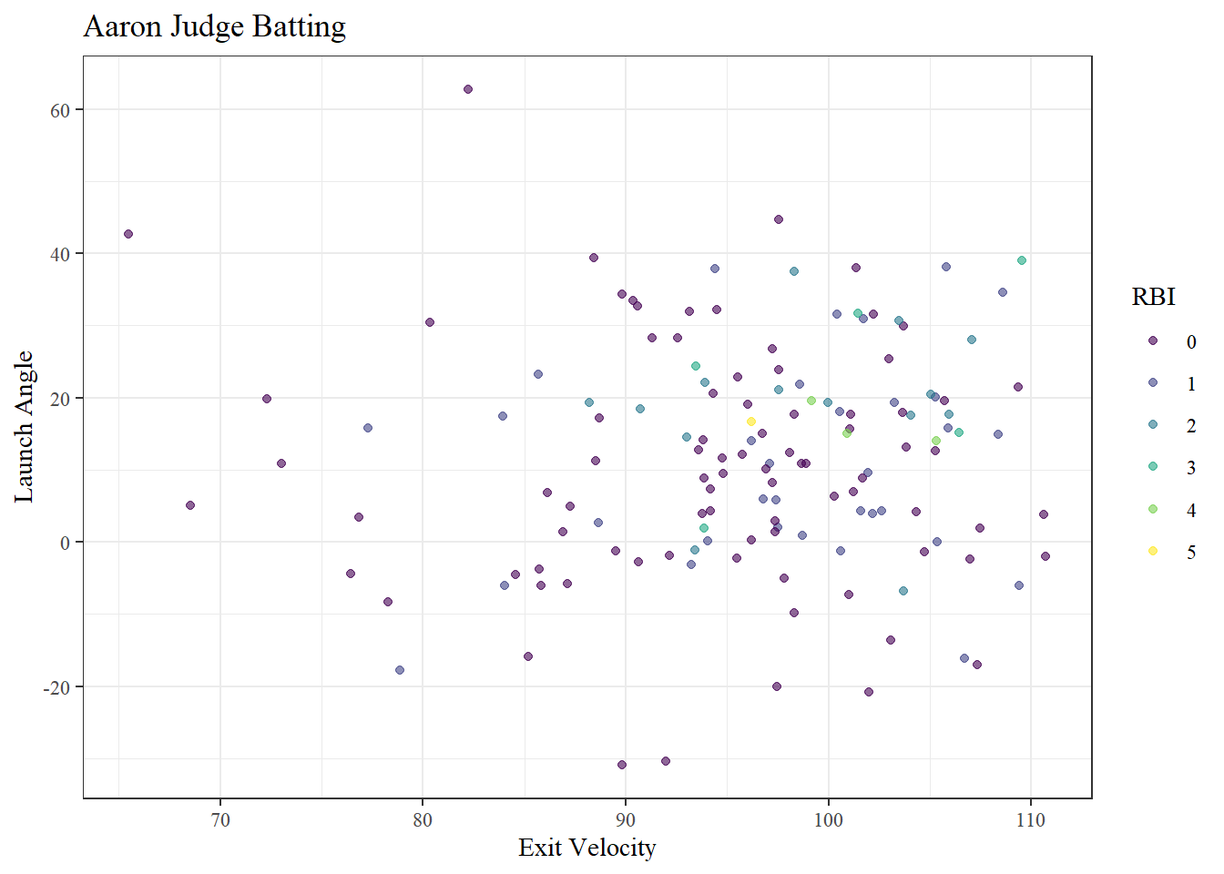
Both of these functions require input of ‘playerid’ and ‘year’. To find a player’s playerid search them on the FanGraphs website. The playerid is the numbers after the player’s name in the URL. For example, to find Aaron Judge’s playerid look at his page: https://www.fangraphs.com/players/aaron-judge/15640/stats?position=OF. Aaron Judge’s FanGraphs player id is 15640.

judge <- fg_batter_game_logs(playerid = 15640, year = 2021)

This produces a data frame with 245 variables. Each row is a different game played within the 2021 season.

judge_filtered <- judge %>% 
  dplyr::select(PlayerName, Date, Opp, Pos, AB:H, HR:BB, SO, `BB%`:BABIP, wOBA, EV:`HardHit%`)

PlayerName	Date	Opp	Pos	AB	PA	H	HR	R	RBI	BB	SO	BB%	K%	BB/K	OBP	SLG	OPS	ISO	BABIP	wOBA	EV	LA	Barrels	Barrel%	maxEV	HardHit	HardHit%
Aaron Judge	2021-05-16	@BAL	DH	3	4	2	1	2	1	1	0	0.25	0.0000000	1.0	0.7500000	1.666667	2.4166667	1.0000000	0.5000000	0.8943226	88.67112	2.635370	1	0.3333333	114.7070	1	0.3333333
Aaron Judge	2021-04-30	DET	RF	4	4	2	2	2	5	0	0	0.00	0.0000000	0.0	0.5000000	2.000000	2.5000000	1.5000000	0.0000000	1.0032593	96.17970	16.673782	1	0.2500000	111.2630	2	0.5000000
Aaron Judge	2021-06-17	@TOR	RF	4	5	1	0	0	0	1	2	0.20	0.4000000	0.5	0.4000000	0.250000	0.6500000	0.0000000	0.5000000	0.3141544	91.98772	-30.357954	0	0.0000000	104.8930	1	0.5000000
Aaron Judge	2021-05-27	TOR	DH	3	3	0	0	0	0	0	1	0.00	0.3333333	0.0	0.0000000	0.000000	0.0000000	0.0000000	0.0000000	0.0000000	93.58981	12.780601	0	0.0000000	100.6680	1	0.5000000
Aaron Judge	2021-09-01	@LAA	RF	3	4	2	1	1	1	1	1	0.25	0.2500000	1.0	0.7500000	1.666667	2.4166667	1.0000000	1.0000000	0.8943226	105.28107	20.101276	1	0.5000000	110.0080	2	1.0000000
Aaron Judge	2021-08-21	MIN	CF-RF	3	4	0	0	0	0	1	1	0.25	0.2500000	1.0	0.2500000	0.000000	0.2500000	0.0000000	0.0000000	0.1729291	102.22653	31.566599	0	0.0000000	109.9630	1	0.5000000
Aaron Judge	2021-06-03	TBR	DH	4	4	1	0	0	0	0	0	0.00	0.0000000	0.0	0.2500000	0.250000	0.5000000	0.0000000	0.2500000	0.2197638	88.41893	39.330715	1	0.2500000	115.1100	1	0.2500000
Aaron Judge	2021-08-11	@KCR	DH	5	5	2	0	1	1	0	1	0.00	0.2000000	0.0	0.4000000	0.400000	0.8000000	0.0000000	0.5000000	0.3516221	96.19725	13.988741	0	0.0000000	108.6280	3	0.7500000
Aaron Judge	2021-05-11	@TBR	RF	4	4	2	1	1	1	0	0	0.00	0.0000000	0.0	0.5000000	1.250000	1.7500000	0.7500000	0.3333333	0.7213935	101.92689	9.627525	1	0.2500000	116.1330	3	0.7500000
Aaron Judge	2021-08-17	BOS	RF	3	4	0	0	1	0	1	2	0.25	0.5000000	0.5	0.2500000	0.000000	0.2500000	0.0000000	0.0000000	0.1729291	97.43213	-20.110865	0	0.0000000	97.4321	1	1.0000000
Aaron Judge	2021-04-06	BAL	RF	5	5	3	1	1	4	0	0	0.00	0.0000000	0.0	0.6000000	1.200000	1.8000000	0.6000000	0.5000000	0.7529258	100.91077	15.009117	1	0.2000000	110.8720	3	0.6000000
Aaron Judge	2021-08-29	@OAK	RF	4	4	0	0	0	0	0	0	0.00	0.0000000	0.0	0.0000000	0.000000	0.0000000	0.0000000	0.0000000	0.0000000	89.52336	-1.241035	0	0.0000000	107.3030	1	0.2500000
Aaron Judge	2021-07-06	@SEA	RF	6	6	2	0	1	1	0	1	0.00	0.1666667	0.0	0.3333333	0.500000	0.8333333	0.1666667	0.4000000	0.3534503	97.07851	10.806757	1	0.2000000	113.9140	3	0.6000000
Aaron Judge	2021-08-28	@OAK	CF	4	4	3	1	1	2	0	0	0.00	0.0000000	0.0	0.7500000	1.750000	2.5000000	1.0000000	0.6666667	1.0318051	105.02797	20.398167	3	0.7500000	111.5450	4	1.0000000
Aaron Judge	2021-05-30	@DET	RF	4	5	1	0	1	0	1	2	0.20	0.4000000	0.5	0.4000000	0.500000	0.9000000	0.2500000	0.5000000	0.3866726	98.31427	17.690056	0	0.0000000	108.3180	1	0.5000000

Leaderboards

To access leaderboards for pitchers: fg_pitcher_leaders() To access leaderboards for pitchers: fg_batter_leaders()

The arguments are ‘x’ for the first season of interest, ‘y’ for the last season of interest, ‘league’, and ‘pitcher_type’ (default is “pit” for all pitchers, other options are “sta” for starters and “rel” for relievers). There are additional optional arguments: ‘ind’, which specifies if if the data should look at one season or over many, and ‘league’, which determines if players must meet a certain qualification to be included (plate appearances for batters and innings per game for pitchers).

pitch_leaders <- fg_pitcher_leaders(x = 2020, y = 2022)

The resulting data frame has 303 variables.

pl_filtered <- pitch_leaders %>% 
  dplyr::select(playerid:G, IP:BB, SO, Pitches, AVG:BABIP, WAR:Dollars)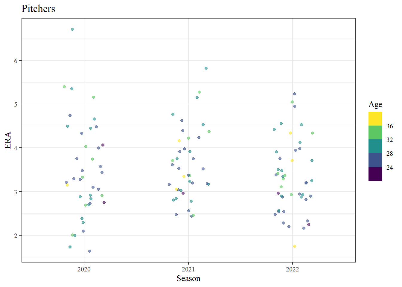

Accessing data from baseballr gives over double the amount of observations and hundreds of more variables.

There are also FanGraphs functions that can scrape park factors.