Lahman
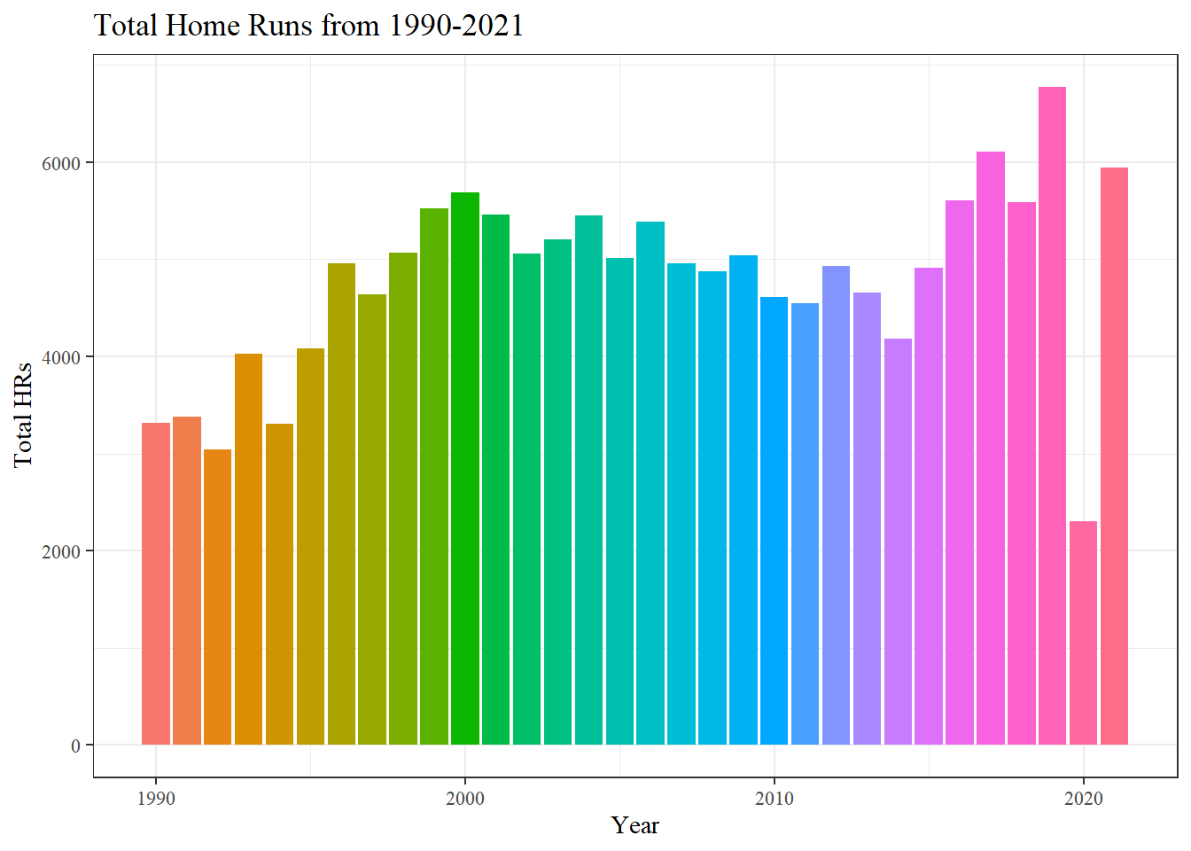
Batting %>%
  group_by(yearID) %>%
  summarize(totalHR = sum(HR)) %>%
  filter(yearID >= 1990) %>%
  ggplot(aes(x = yearID, y = totalHR, fill = factor(yearID))) +
  geom_col() +
  labs(title = "Total Home Runs from 1990-2021", x = "Year", y = "Total HRs") +
  theme_bw() +
  theme(text = element_text(family = "serif")) +
  theme(legend.position = "none")
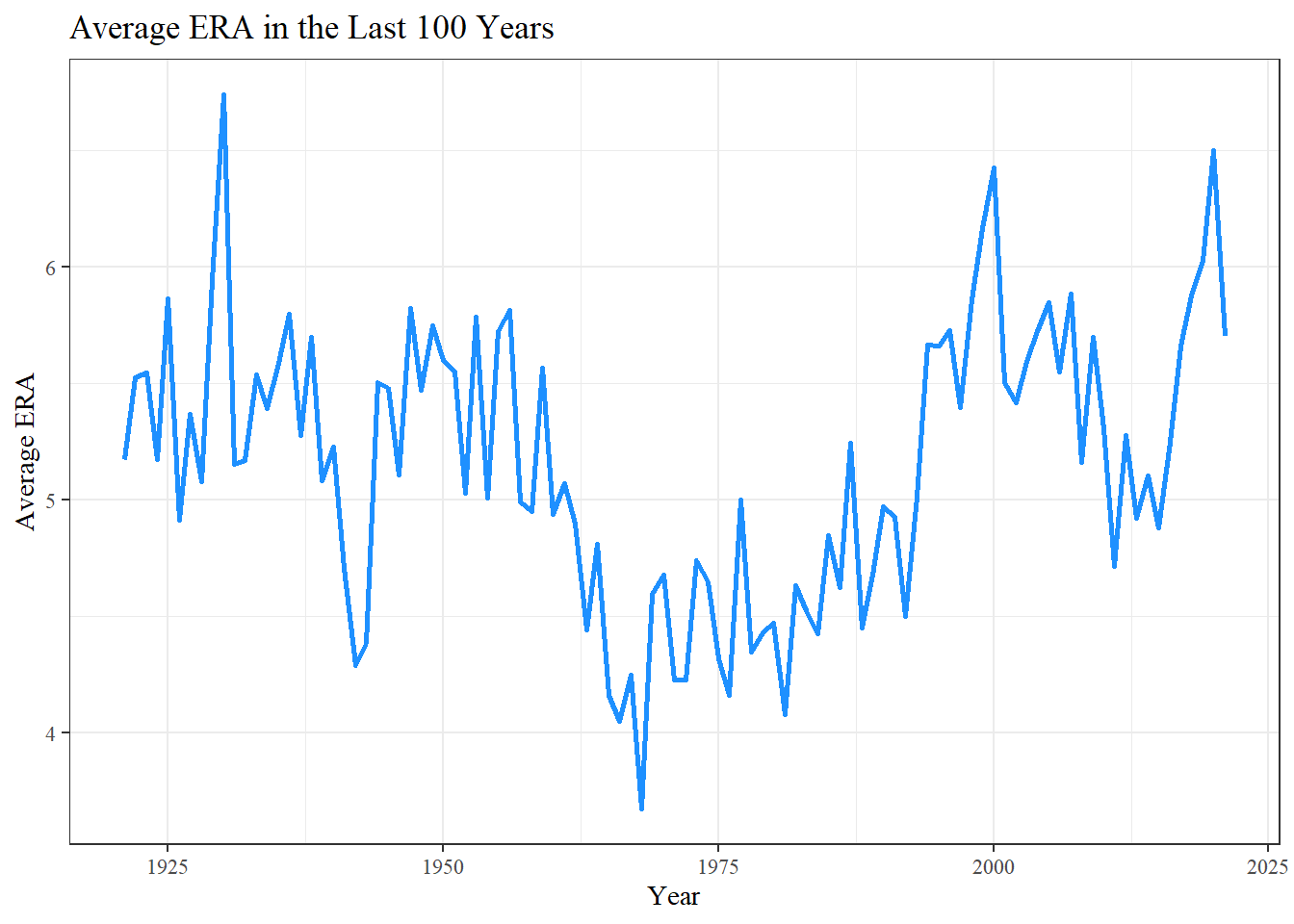
Pitching %>%
  group_by(yearID) %>%
  filter(yearID >= 1921, !is.na(ERA)) %>%
  summarize(avgERA = mean(ERA)) %>%
  ggplot(aes(x = yearID, y = avgERA)) +
  geom_line(size = 1, color = "dodgerblue") +
  labs(title = "Average ERA in the Last 100 Years",
       x = "Year", y = "Average ERA") +
  theme_bw() +
  theme(text = element_text(family = "serif"))
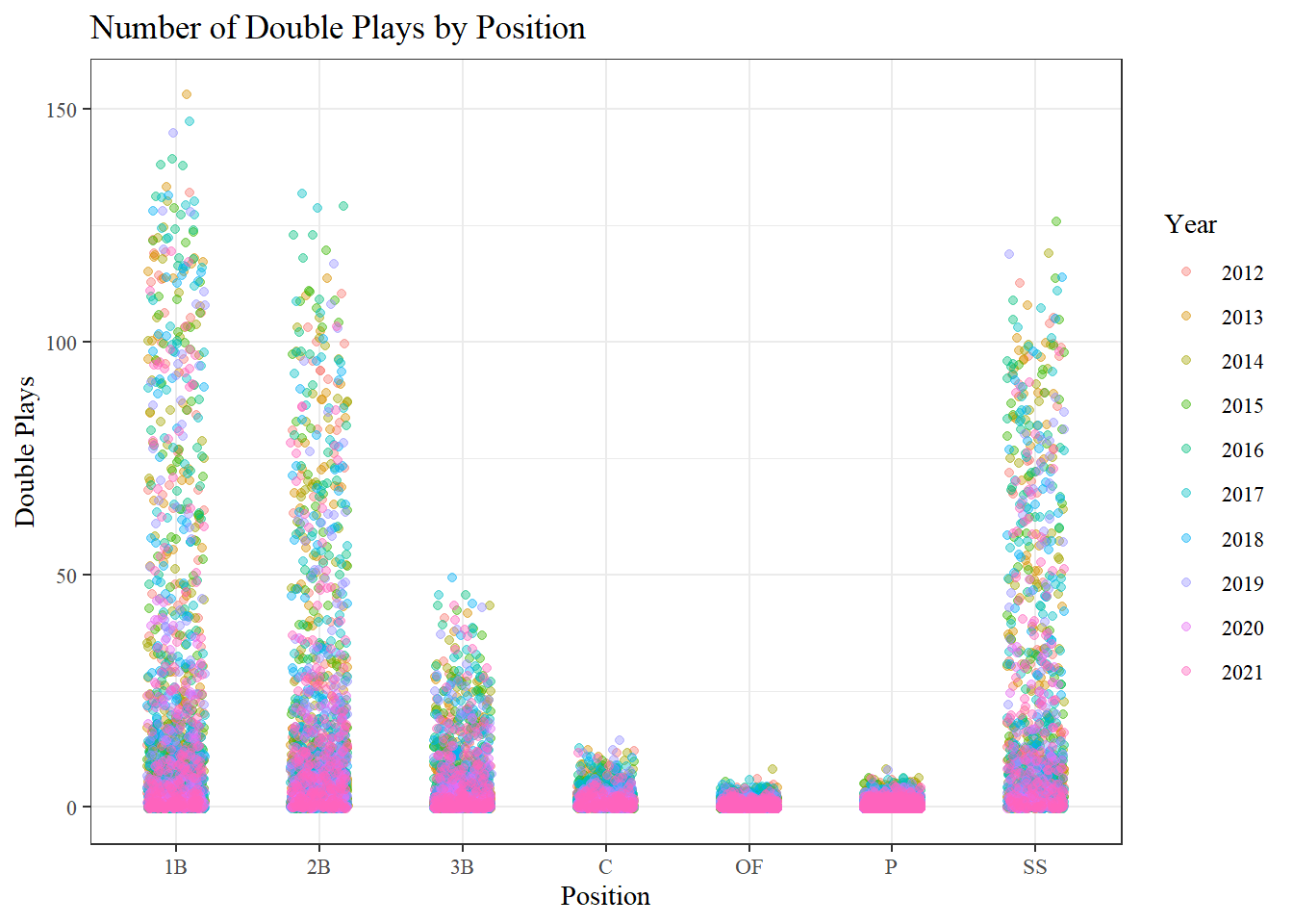
Fielding %>%
  filter(yearID >= 2012) %>%
  ggplot(aes(x = factor(POS), y = DP)) +
  geom_jitter(alpha = 0.4, aes(color = factor(yearID)),
              position = position_jitter(0.2)) +
  labs(title = "Number of Double Plays by Position",
       x = "Position", y = "Double Plays", color = "Year") +
  theme_bw() +
  theme(text = element_text(family = "serif"))
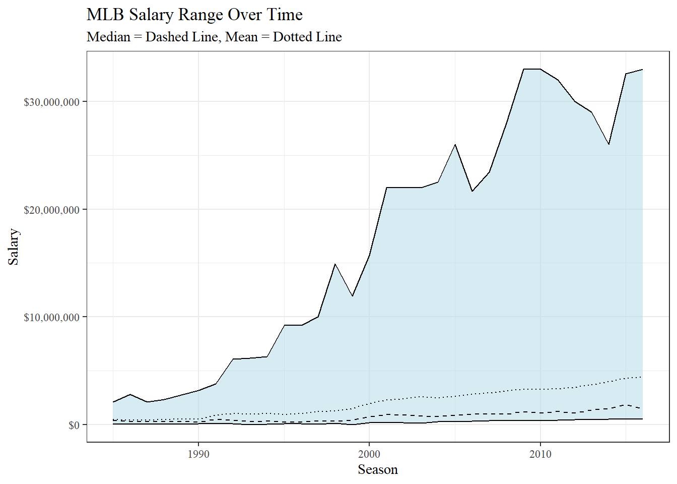
Salaries %>%
  group_by(yearID) %>%
  summarize(Low = min(salary), Median = median(salary),
                     Mean = mean(salary), High = max(salary)) %>%
  ggplot(aes(x = yearID)) +
  geom_ribbon(aes(ymin = Low, ymax = High),
                        fill = "lightblue", color = "black", alpha = 0.5) +
  geom_line(aes(y = Median), color = "black", linetype = "dashed") +
  geom_line(aes(y = Mean), color = "black", linetype = "dotted") +
  scale_y_continuous(labels = scales::label_dollar()) +
  labs(title = "MLB Salary Range Over Time",
          subtitle = "Median = Dashed Line, Mean = Dotted Line",
          y = "Salary",
          x = "Season") +
  theme_bw() +
  theme(text = element_text(family = "serif"))
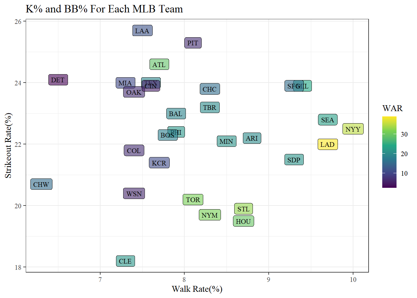
FanGraphs
fg_update %>%
  ggplot(aes(x = BB_rate, y = K_rate, label = Team, fill = WAR)) +
  geom_label(alpha = 0.6, size = 3, family = "serif") +
  labs(title = "K% and BB% For Each MLB Team",
       x = "Walk Rate(%)", y = "Strikeout Rate(%)") +
  scale_fill_viridis_c() +
  theme_bw() +
  theme(text = element_text(family = "serif"))
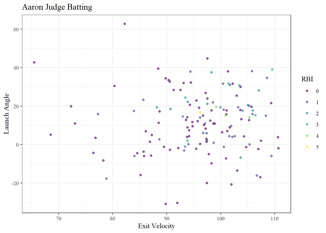
judge_filtered %>%
  ggplot(aes(x = EV, LA, color = factor(RBI))) +
  geom_point(alpha = 0.6) +
  labs(title = "Aaron Judge Batting",
       x = "Exit Velocity", y = "Launch Angle", color = "RBI") +
  scale_color_viridis_d() +
  theme_bw() +
  theme(text = element_text(family = "serif"))
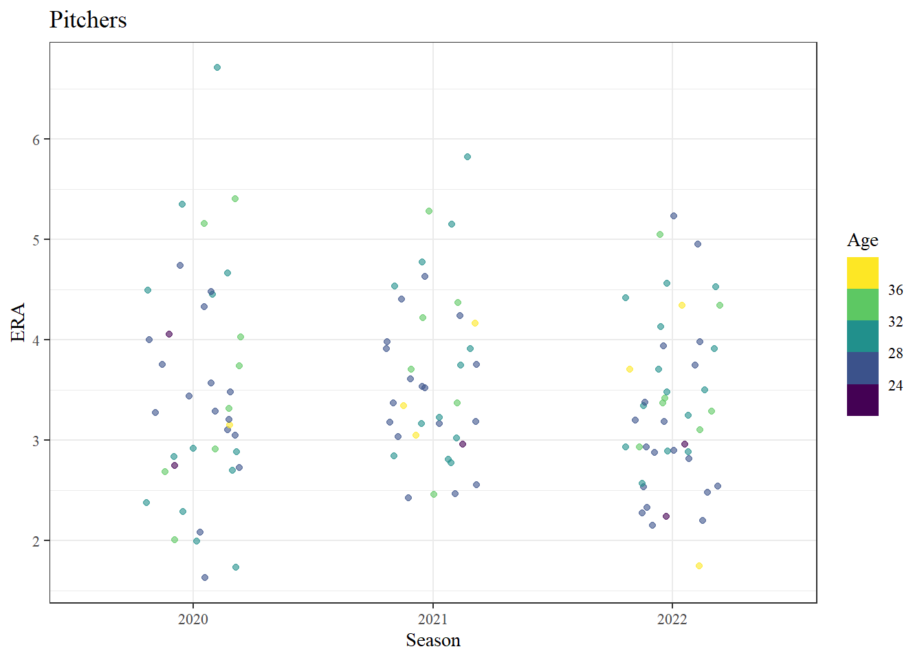
pl_filtered %>%
  ggplot(aes(x = factor(Season), y = ERA)) +
  geom_jitter(alpha = 0.6, aes(color = Age),
              position=position_jitter(0.2)) +
  labs(title = "Pitchers", x = "Season") +
  scale_color_viridis_b() +
  theme_bw() +
  theme(text = element_text(family = "serif"))
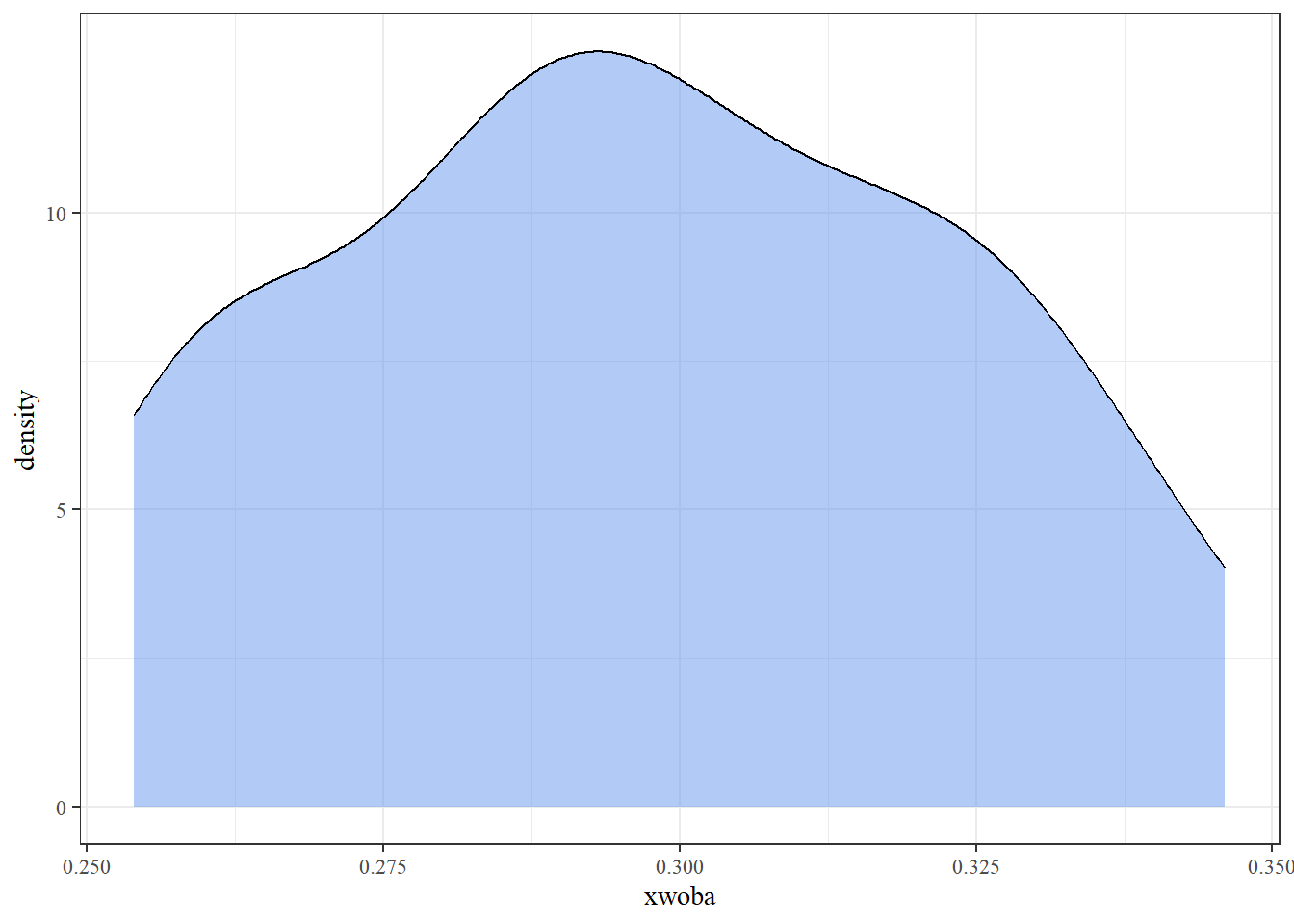
Statcast
sc_download %>%
  ggplot(aes(x = xwoba)) +
  geom_density(fill = "cornflowerblue", alpha = .5) +
  theme_bw() +
  theme(text = element_text(family = "serif"))
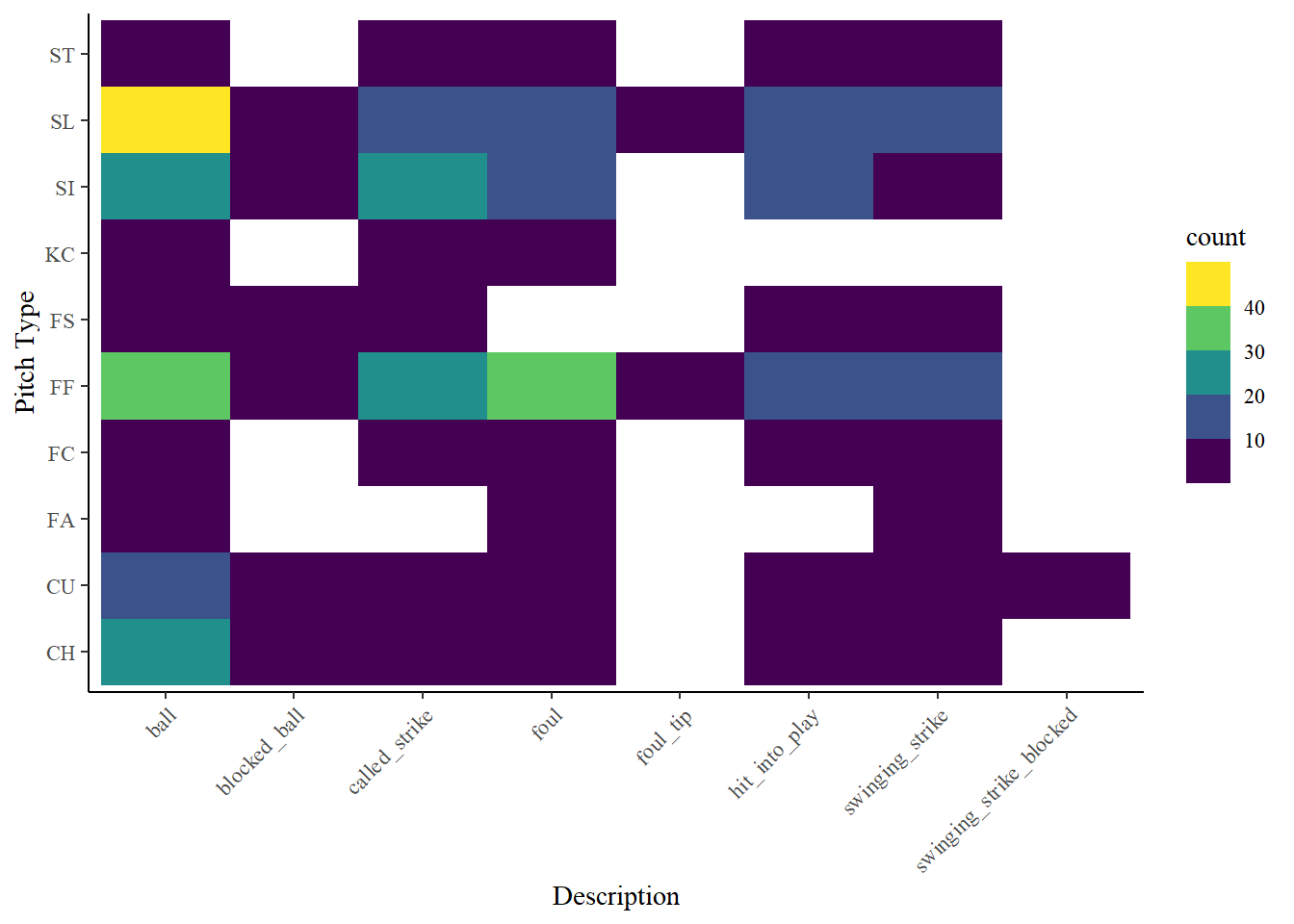
judge_sc %>%
  group_by(description, pitch_type) %>%
  summarize(count = n()) %>%
  ggplot(aes(x = description, y = pitch_type, fill = count)) +
  geom_tile() +
  labs(x = "Description", y = "Pitch Type", color = "Release Speed") +
  scale_fill_viridis_b() +
  theme_classic() +
  theme(axis.text.x = element_text(angle = 45, hjust = 1)) +
  theme(text = element_text(family = "serif"))
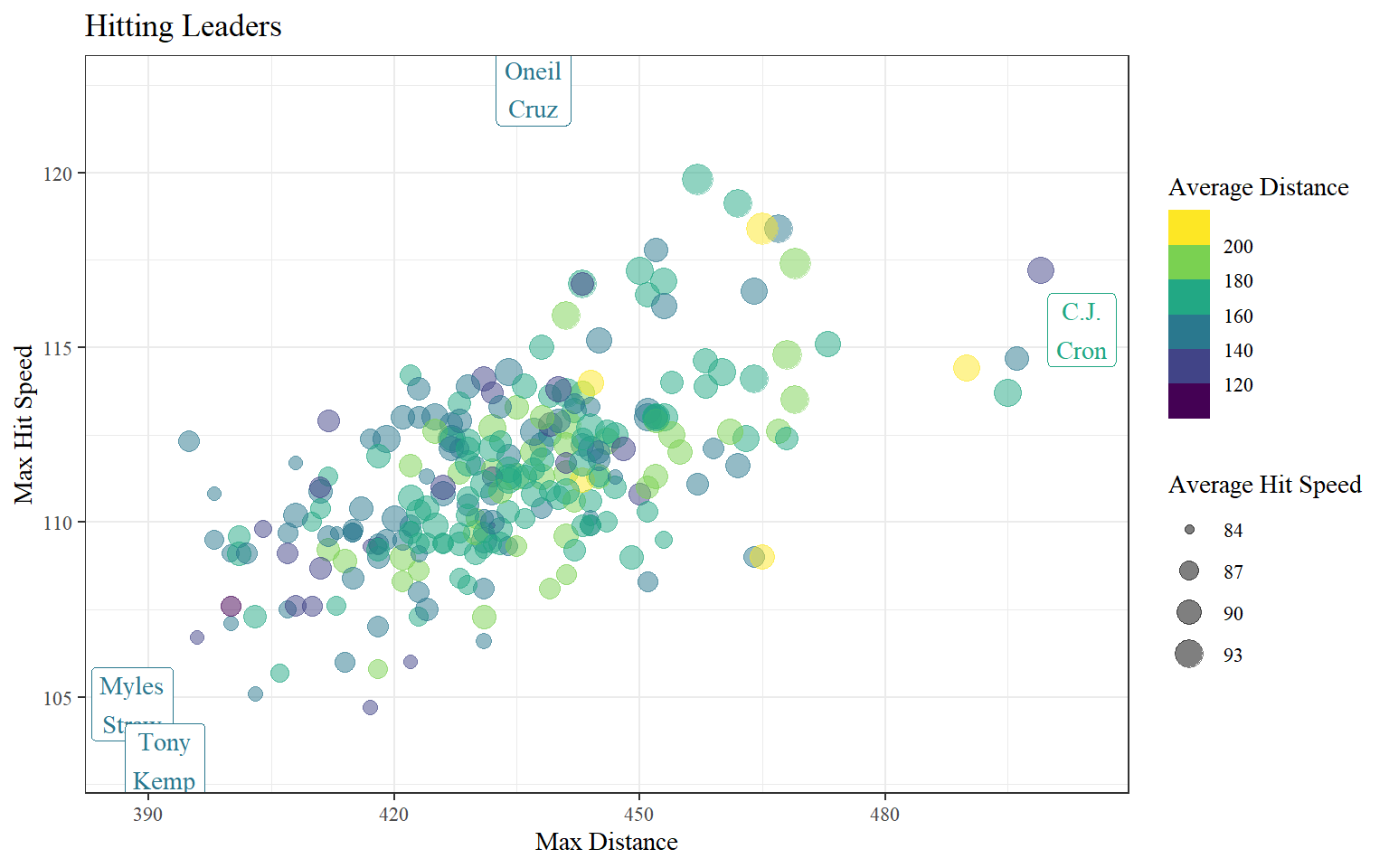
sc_lead_evb %>%
  group_by(player_id) %>%
  ggplot(aes(x = max_distance, y = max_hit_speed, color = avg_distance)) +
  geom_point(alpha = .5, aes(size = avg_hit_speed)) +
  geom_label(data = sc_lead_evb %>%
               filter(max_distance %in% range(max_distance) |
                        max_hit_speed %in% range(max_hit_speed)),
             aes(label = paste(first_name, last_name, sep = "\n")),
             show.legend = FALSE, family = "serif") +
  labs(title = "Hitting Leaders", x = "Max Distance", y = "Max Hit Speed",
       color = "Average Distance", size = "Average Hit Speed") +
  scale_color_viridis_b() +
  theme_bw() +
  theme(text = element_text(family = "serif"))
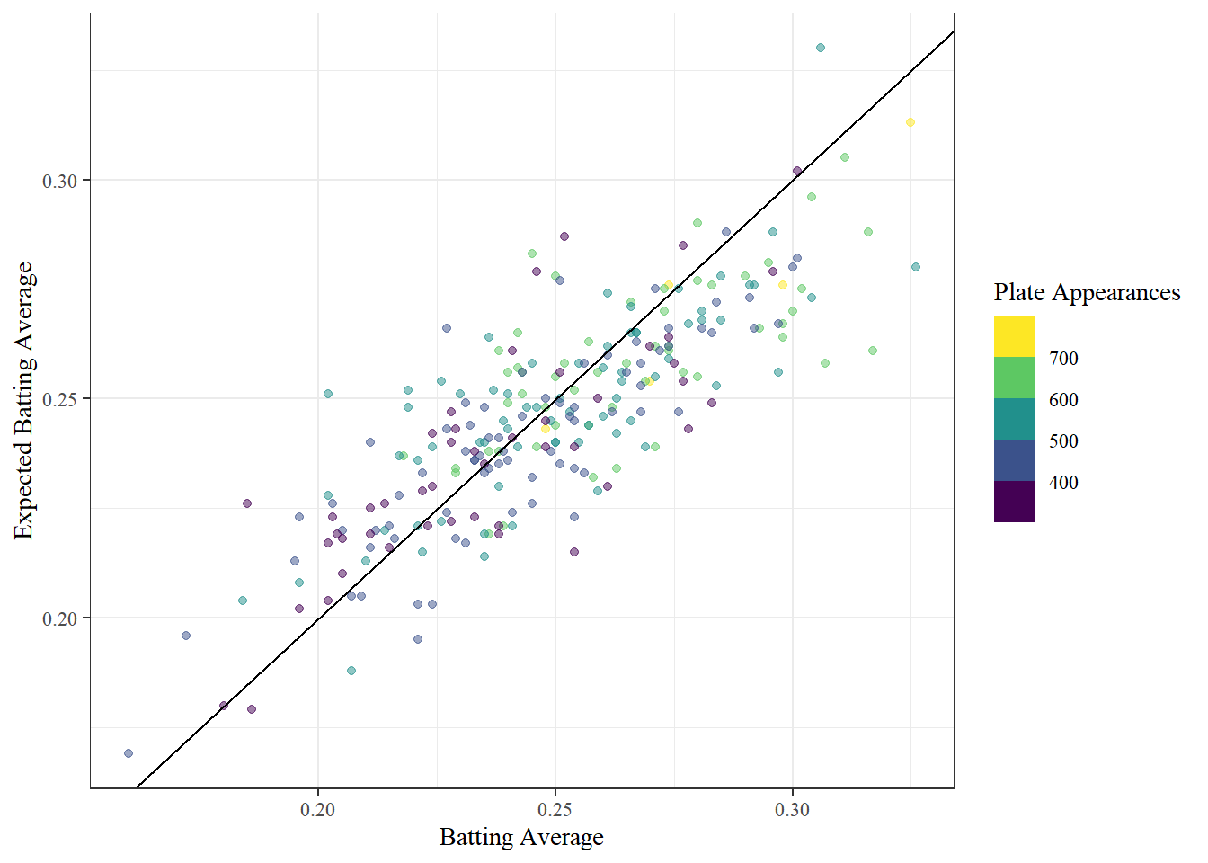
sc_lead_exp %>%
  ggplot(aes(x = ba, y = est_ba, color = pa)) +
  geom_point(alpha = .5) +
  geom_abline() +
  labs(x = "Batting Average", y = "Expected Batting Average",
       color = "Plate Appearances") +
  scale_color_viridis_b() +
  theme_bw() +
  theme(text = element_text(family = "serif"))