7 Modeling
7.1 Simple Linear Regression
Predicting Winning Percentage
For this section we will be using the Teams table.
team_pred <- Teams %>%
  filter(yearID >= 2012, yearID < 2020)
Say we want to predict winning percentage using a team’s run differential. To do this we need to create two new variables: run differential (RD) and winning percentage (WPCT). Run differential is calculated with runs scored (R) and runs allowed (RA). Calculating winning percentage requires the amount of wins and losses.
team_pred <- team_pred %>%
  mutate(RD = R - RA,
         WPCT = W / (W + L))
Now it’s time to build the model. The lm() function is used to fit linear models. It requires a formula, following the format: response ~ predictor(s). A response variable is the variable we are trying to predict. Predictor variables are used to make predictions. In this example, we will predict a team’s winning percentage (response) using its run differential (predictor).
model1 <- lm(WPCT ~ RD, data = team_pred)
model1
##
## Call:
## lm(formula = WPCT ~ RD, data = team_pred)
##
## Coefficients:
## (Intercept) RD
## 0.4999830 0.0006089The general equation of a simple linear regression line is: \(\hat{y} = b_0 + b_1 x\). The symbols have the following meaning:
- \(\hat{y}\) = predicted value of the response variable
- \(b_0\) = estimated y-intercept for the line
- \(b_1\) = estimated slope for the line
- x = predictor value to plug in
This output provides us with an equation we can use to predict a team’s winning percentage based on their run differential:
\[\text{Predicted Win Pct} = 0.500 + 0.00061 * \text{Run Diff}\]
The estimated y-intercept for this model is 0.500. This means that we would predict a winning percentage of 0.500 for a team with a run differential of 0. In other words, teams who give up and score the same number of runs are predicted to be average. This makes a lot of sense for this example, but we will see later that y-intercept interpretations aren’t always applicable like this.
The slope for this model is 0.0006267. There are 162 games in the MLB regular season. If we multiple the slope by 162 we get 0.1015, which equates to 1/10th of a win. For each additional difference the predicted wins goes up by 0.0006. This works out to about 0.1 wins.
The estimate slope for our line is 0.00061. This tells us that our predicted winning percentage increases by 0.00061 for each additional run a team scores (or each fewer run they allow). Over a 162 game season, a change in winning percentage of 0.00061 is equivalent to around \(162 * 0.00061 = 0.1\) wins. In other words, an increase of around 10 runs scored (or prevented) is associated with around 1 more win in a season.
The summary() function can give us some additional information about our linear regression model.
summary(model1)##
## Call:
## lm(formula = WPCT ~ RD, data = team_pred)
##
## Residuals:
## Min 1Q Median 3Q Max
## -0.060481 -0.016448 0.000136 0.014840 0.081565
##
## Coefficients:
## Estimate Std. Error t value Pr(>|t|)
## (Intercept) 5.000e-01 1.630e-03 306.74 <2e-16 ***
## RD 6.089e-04 1.414e-05 43.05 <2e-16 ***
## ---
## Signif. codes: 0 '***' 0.001 '**' 0.01 '*' 0.05 '.' 0.1 ' ' 1
##
## Residual standard error: 0.02525 on 238 degrees of freedom
## Multiple R-squared: 0.8862, Adjusted R-squared: 0.8857
## F-statistic: 1854 on 1 and 238 DF, p-value: < 2.2e-16Another important thing to look at is the p-value. A p-value tells us how likely certain results would be to occur if “nothing was going on”. We often compare a p-value to a pre-chosen significance level, alpha, to decide if our results would be unusual in a world where our variables weren’t related to one another. The most frequently used significance level is alpha = 0.5. Our model’s p-value is less than 2.2e-16, or 0.00000000000000022, which is much smaller than alpha. This suggests that run differential is helpful in predicting winning percentage because results like this are incredibly unlikely to occur if the two variables are not related.
R-squared values are used to describe how well the model fits the data. In this model, the R-squared value is 0.8862. This is saying that around 88.6% of variability in team winning percentage is explained by run differential.
This should not be the exclusive method to assess model fit, but it helps give us a good idea.
To visualize this data we can make a scatter plot and fit a line using geom_smooth(). If no method is specified, R will automatically fit the model it thinks is best. Since we fit a linear model above, the method should be “lm”.
team_pred %>%
  ggplot(aes(x = RD, y = WPCT)) +
  geom_point(alpha = 0.5) +
  geom_smooth(method = "lm") +
  theme_bw() +
theme(text = element_text(family = "serif")) 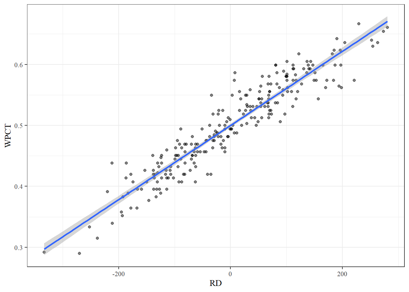
7.2 Multiple Linear Regression
Linear Weights
We are going to predict runs using singles, doubles, triples, homeruns, walks, hit-by-pitches, strikeouts, non-strikeouts, stolen bases,caught stealing, and sacrifice flies.
First, we need to create a variable for singles (‘X1B’) and a variable for non-strikeouts (‘nonSO’).
team_pred <- team_pred %>%
  mutate(X1B = H - X2B - X3B - HR,
         nonSO = AB - H - SO)
model2 <- lm(R ~ X1B + X2B + X3B + HR + BB + HBP + SO + nonSO + SB + CS + SF,
data = team_pred)
summary(model2)##
## Call:
## lm(formula = R ~ X1B + X2B + X3B + HR + BB + HBP + SO + nonSO +
## SB + CS + SF, data = team_pred)
##
## Residuals:
## Min 1Q Median 3Q Max
## -47.81 -14.37 0.89 13.04 69.67
##
## Coefficients:
## Estimate Std. Error t value Pr(>|t|)
## (Intercept) -81.21901 148.24516 -0.548 0.58432
## X1B 0.39787 0.03233 12.307 < 2e-16 ***
## X2B 0.85061 0.06261 13.586 < 2e-16 ***
## X3B 1.03933 0.17326 5.999 7.74e-09 ***
## HR 1.46736 0.04932 29.753 < 2e-16 ***
## BB 0.27187 0.02782 9.772 < 2e-16 ***
## HBP 0.42777 0.10061 4.252 3.09e-05 ***
## SO -0.07631 0.03220 -2.370 0.01864 *
## nonSO -0.06349 0.03324 -1.910 0.05740 .
## SB 0.19421 0.06119 3.174 0.00171 **
## CS -0.48760 0.21522 -2.266 0.02441 *
## SF 0.54241 0.20892 2.596 0.01004 *
## ---
## Signif. codes: 0 '***' 0.001 '**' 0.01 '*' 0.05 '.' 0.1 ' ' 1
##
## Residual standard error: 21.41 on 228 degrees of freedom
## Multiple R-squared: 0.9264, Adjusted R-squared: 0.9228
## F-statistic: 260.7 on 11 and 228 DF, p-value: < 2.2e-16Most of the p-values from this model have stars next to them. ** is significant at alpha = 0.001. *** is significant at alpha = 0.0001. The intercept’s p-value is the only one without stars. A p-value of 0.205166 suggests that we may not need the the intercept. This makes sense since a team that does none of these things (the predictor variables) would score 0 runs.
Now let’s try fitting a model with no intercept. We can accomplish this by putting “- 1” at the of the model equation.
model2 <- lm(R ~ X1B + X2B + X3B + HR + BB + HBP + SO + nonSO + SB + CS + SF - 1,
             data = team_pred)
summary(model2)
##
## Call:
## lm(formula = R ~ X1B + X2B + X3B + HR + BB + HBP + SO + nonSO +
## SB + CS + SF - 1, data = team_pred)
##
## Residuals:
## Min 1Q Median 3Q Max
## -48.01 -13.86 0.80 13.12 68.72
##
## Coefficients:
## Estimate Std. Error t value Pr(>|t|)
## X1B 0.39067 0.02949 13.249 < 2e-16 ***
## X2B 0.85129 0.06250 13.620 < 2e-16 ***
## X3B 1.03715 0.17295 5.997 7.78e-09 ***
## HR 1.46017 0.04747 30.763 < 2e-16 ***
## BB 0.26895 0.02726 9.865 < 2e-16 ***
## HBP 0.42674 0.10043 4.249 3.13e-05 ***
## SO -0.09294 0.01073 -8.662 8.47e-16 ***
## nonSO -0.08079 0.01037 -7.792 2.28e-13 ***
## SB 0.19451 0.06109 3.184 0.00166 **
## CS -0.51912 0.20707 -2.507 0.01287 *
## SF 0.53241 0.20780 2.562 0.01105 *
## ---
## Signif. codes: 0 '***' 0.001 '**' 0.01 '*' 0.05 '.' 0.1 ' ' 1
##
## Residual standard error: 21.38 on 229 degrees of freedom
## Multiple R-squared: 0.9992, Adjusted R-squared: 0.9991
## F-statistic: 2.453e+04 on 11 and 229 DF, p-value: < 2.2e-16This model’s p-value is 2.2e-16, which is incredibly small. The R-squared value is 0.9992, meaning that 99.9% of variability in runs is explained by these 10 variables.
Here is a table of the of each MLR variable and their slope:
kable(model2$coefficients, col.names = "Coefficient") %>%
kable_styling("striped", full_width = FALSE)| Coefficient | |
|---|---|
| X1B | 0.3906674 |
| X2B | 0.8512873 |
| X3B | 1.0371486 |
| HR | 1.4601679 |
| BB | 0.2689488 |
| HBP | 0.4267400 |
| SO | -0.0929440 |
| nonSO | -0.0807918 |
| SB | 0.1945057 |
| CS | -0.5191153 |
| SF | 0.5324062 |
The coefficient for stolen bases is 0.1945. This means that a team will score 0.1945 runs for every base they steal, given that all other variables remain constant. A coefficient of -0.5191 for caught stealing is saying that the number of runs will decrease by -0.5191 for every time the team is caught stealing.
To see how good this model is we will plot the predicted runs against the actual runs. The line represents a perfect model.
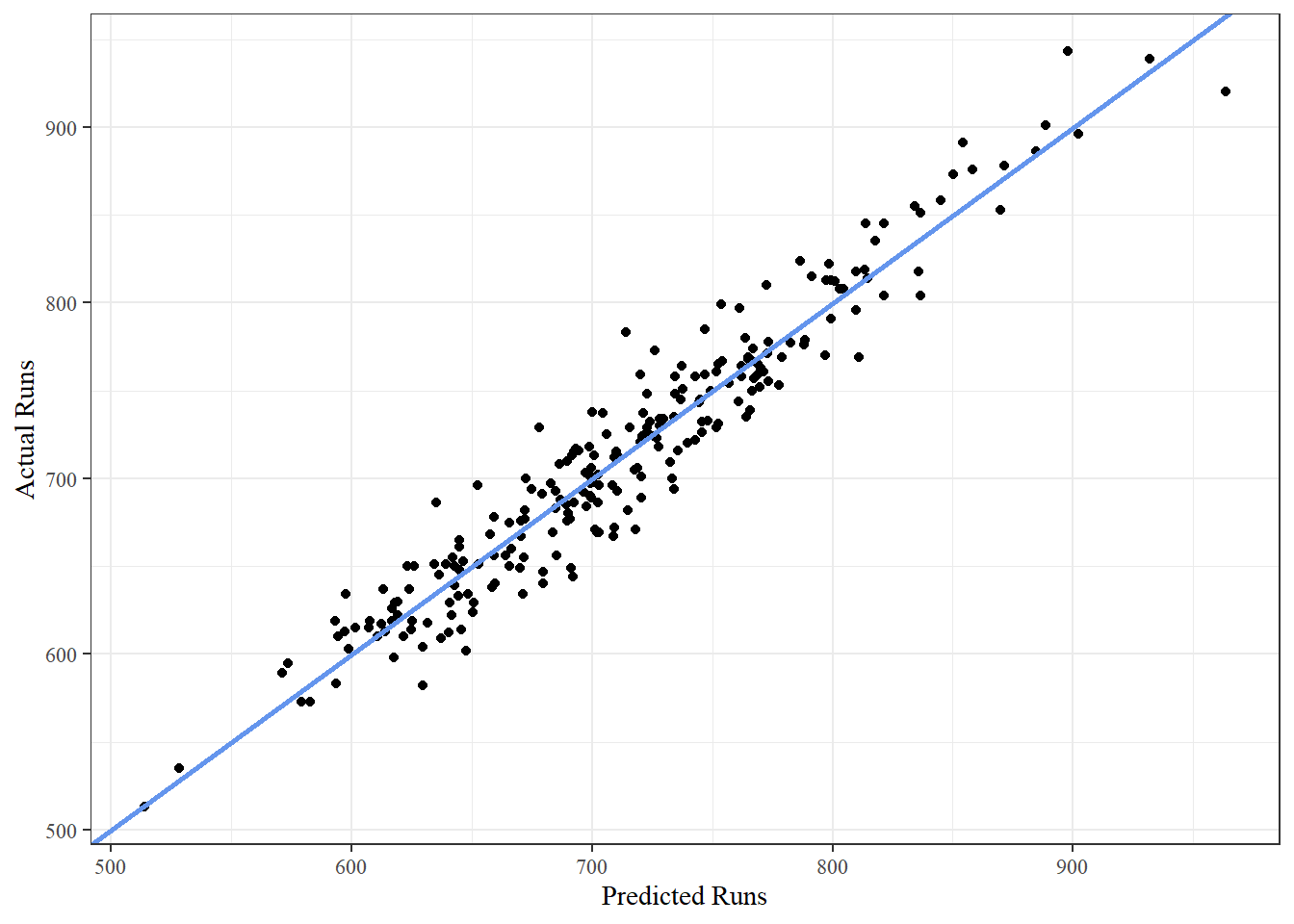
The points stay close to the line, which indicates that the model fits the data very well. This supports the same conclusion as the R-squared value.