Chapter 1 The ecology behind species-habitat-association models
1.1 Objectives
To define what we mean by habitat and its constituent environmental variables.
To distinguish between the effect of habitat on fitness and on species distribution.
To identify the behavioral and demographic drivers of SHAs.
To introduce an appropriate null model for species-habitat associations (SHAs) that encapsulates fundamental concepts such as the Ideal free distribution (IDF), the pseudo-equilibrium assumption and the niche.
To outline the biological mechanisms that can violate the null model for SHAs.
To synthesize the state of the art in the currently best developed methodology for quantifying SHAs using species distribution models (SDMs).
1.2 How do living beings “see” the world around them?
Individuals experience the world around them in different ways, but what ultimately matters for an organism’s fitness and distribution is whether it has a positive, negative or ambivalent relationship with aspects of its environment. This trichotomy allows us to classify environmental variables into resources, risks and conditions. Although there is clearly some ambiguity in classifying environmental variables into these three categories, they will facilitate the model development outlined in Chapter 2. Furthermore, these three classes will provide us the opportunity to present different examples of the environmental variables driving species-habitat associations.
1.2.1 Resources
Resources are substances, objects or places in the environment required by an organism for normal growth, maintenance, and reproduction, and therefore resources generally have a positive effect on fitness. Examples of resources for plants are sunlight, carbon dioxide, minerals and water, and for animals are prey, water, and nesting or resting spaces. In overabundance, resources could potentially turn into risks and their effect on fitness may become negative. For example, some food sources consumed by animals contain poisonous substances that may become lethal when consumed in large quantities, or for plants, the photosynthetic machinery can be damaged by too much light. However, most often resources are limited because they are reduced by an organism and its conspecifics or heterospecifics, for example, by consumption or occupancy. Resource limitation leads to inter- or intra-specific competition, which limits species distributions globally and locally. Resource limitation can also lead to a dynamic feedback between resources and consumers, because resources often have their own dynamics.
1.2.2 Risks
Risks are environmental variables that have a negative relationship with fitness by lowering the actual or perceived chances of individual survival or reproduction. Risks may shape distributions by influencing demographic rates (e.g. a predator can cause death and a toxic substance can cause abortion), but the perception of risk by organisms may be just as influential (Laundré, Hernández, & Ripple, 2010). For example, in the case of human encroachment (Ciuti et al., 2012), even as some environmentally hostile anthropogenic activities are waning, the mere presence of humans can maintain entrenched avoidance behaviors by animals and limit their access to valuable resources [the idea of “landscapes of fear”; J. S. Brown, Laundre, & Gurung (1999)]. It is common for risks, like predation pressure, to have a deciding influence on species distributions. For example, intense commercial whaling has led to the extinction of Gray whales in the North Atlantic. While those main threats have now disappeared, Gray whales remain virtually absent in the North Atlantic ocean, despite suitable local conditions (Monsarrat et al. (2015), Fig. 1.1). Also, environments that favor parasites may suppress the distribution of their hosts locally, resulting in the absence of the host species from areas that may otherwise be optimal for their survival (Giannini, Chapman, Saraiva, Alves-dos-Santos, & Biesmeijer, 2013). Despite the potential importance of risk layers in shaping species distributions, they are rarely included in species distribution models because actual and perceived risks tend to be dynamic processes that are difficult to quantify (Palmer, Fieberg, Swanson, Kosmala, & Packer, 2017).
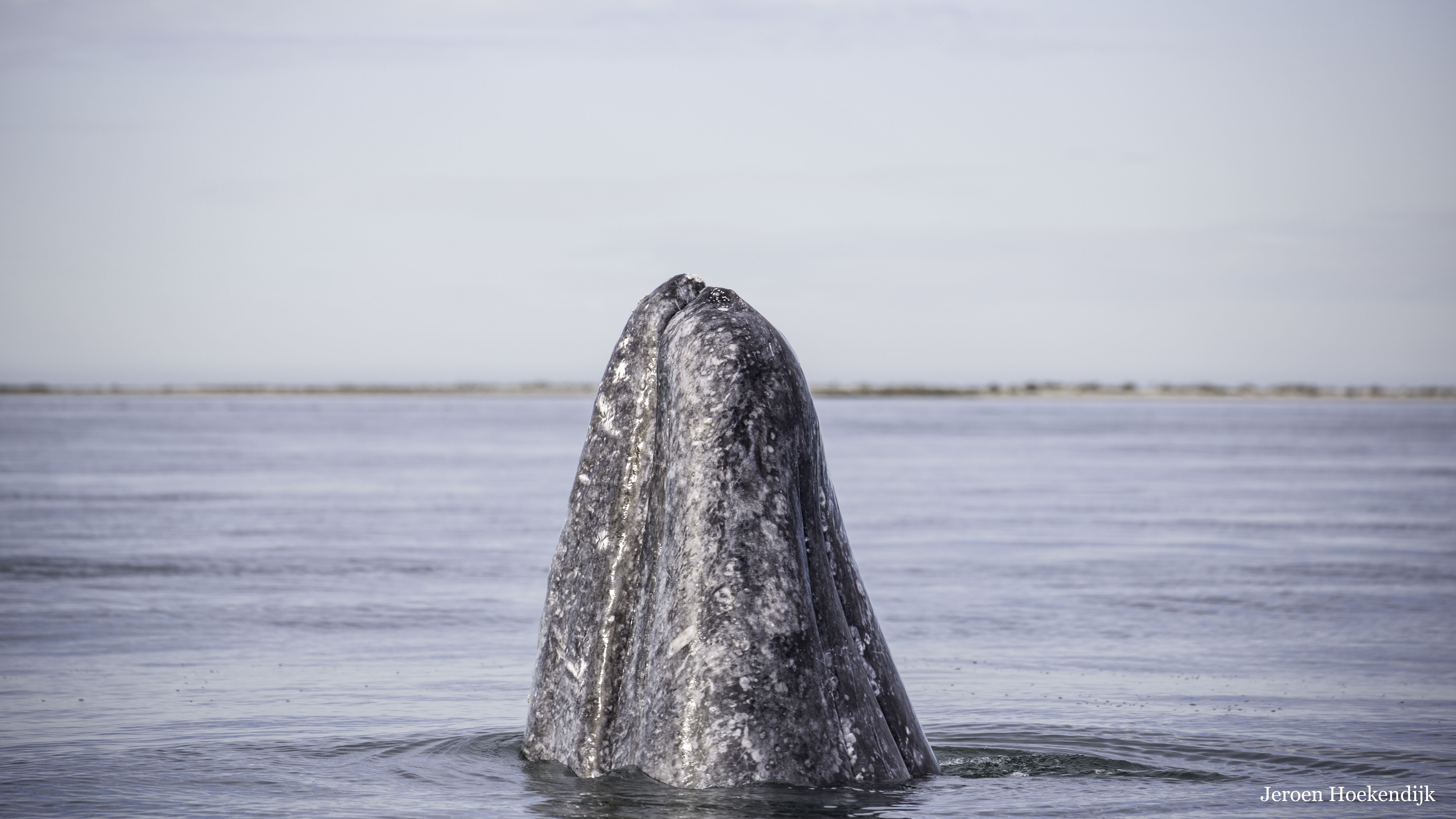
Figure 1.1: Gray whales (Eschrichtius robustus) currently only reside in the Pacific Ocean, but used to live in the Atlantic. Their population became locally extinct in the Atlantic Ocean in the early 18th century, at least partly due to commercial whaling. Apart from the historic risks imposed by whaling, the Atlantic likely remains suitable habitat for gray whales (Monsarrat et al., 2015). Photo: Jeroen Hoekendijk.
1.2.3 Conditions
Conditions are environmental variables (such as ambient temperature, humidity, salinity or pressure) that surround the organism and influence its functioning. Crucially, conditions can have both positive and negative influences on fitness. For example, temperature regulates metabolism (particularly in cold-blooded organisms), and for extreme high or low values (i.e. outside the thermal neutral ‘Goldilocks zone’), organisms may not function properly and die. Although, like resources, conditions may be modified by the actions of organisms [see literature on ecosystem engineers; e.g. Odling-Smee, Laland, & Feldman (2013)], they are generally considered external drivers.
1.2.4 Interactions between resources, risks and conditions
All three classes of environmental variables interact, and this can lead to apparently counter-intuitive effects on species distributions. The resource-risk interaction is nicely captured by the phrase: ‘Is it worth the risk?’ (Joel S. Brown & Kotler, 2004). Predation risks, in particular, may cause organisms to avoid risky habitats despite high resource density (McNamara & Houston, 1987). Sometimes interactions between risks and resources may lead to counter-intuitive effects on species-habitat associations. For example, while populations exposed to risk may have lower survival, those individuals that survive may experience less resource competition, and this may ultimately increase overall population fitness (Van Leeuwen, De Roos, & Persson, 2008). Resource-condition interactions relate to the effect of environmental conditions on the detection and intake of resources. For example, depth and sediment type may influence the accessibility of marine invertebrates to their predators (De Goeij & Honkoop, 2002; Van Gils, Edelaar, Escudero, & Piersma, 2004). An example of a risk-condition interaction is the effect of canopy cover reducing or enhancing the exposure to predation (Joel S. Brown & Kotler, 2004). Finally, all three classes of variables may interact in counter-intuitive ways. For example, although warm-blooded marine mammals need to invest heavily in thermal regulation to avoid the risk of hypothermia, many species of seals and whales are particularly abundant in polar environments. It is believed that their warm-blooded nature allows them to outswim their cold-blooded prey giving them a competitive advantage in colder conditions over other top predators, like sharks (Grady et al., 2019).
1.3 What is a habitat?
Although it is unambiguous that habitat is somehow related to environmental variables, its precise definition in the contemporary ecological literature is rather vague (Dennis, 2012; Kirk et al., 2018). To clarify the concept, we need to answer three questions that can be traced back to ambiguous uses of the term in the literature: 1) Is habitat a place, or a set of circumstances? 2) Should habitat comprise just conditions, or should it also include resources and risks? 3) Is habitat species-specific, or species-independent? Such details of semantics are worth considering because different answers lead to different analytical decisions and interpretations of results.
First, let us consider the possibility of habitat as a region in space. Intuitively, classifying a region in space as a habitat manages to encompass the spatial context in which environmental variables (resources, conditions and risks) are arranged in relation to each other. For instance, from the perspective of an arboreal primate, a single tree is of no value, but a collection of trees in close proximity is home. Equivalently, for a small grazer the availability of short vegetation for food may need to be combined with tall vegetation for cover. These two types of vegetation may not coexist locally, but they must be found in close proximity to be of value to the grazer. Several authors have therefore defined habitat as a suite of resources, risks and environmental conditions, together with their spatial configuration in a landscape (Caughley & Sinclair, 1994; Weddell, 2002). Such a region-specific definition of habitat makes it easier to link habitat to species distribution data collected from the field.
However, a region-specific definition of habitat has several methodological disadvantages. First, it requires us to divide space into discrete parts a-priori, which can be challenging, particularly when multiple, nested spatial scales are relevant for different environmental variables. Second, the appropriate scale of spatial configuration also depends on the species’ mobility and the spatial scales at which it perceives its surroundings. Finally, the environmental makeup of regions in space does not stay constant. It might change daily or seasonally, but also abruptly due to human intervention or natural drivers. So, if we define a habitat as a place, we either have to insist that its composition is static, or we have to allow the environmental properties of “habitat” to change. Overall therefore, although habitats can be mapped onto geographical space and although models should be equipped to understand spatial associations (e.g. in order to capture complementary use of neighboring habitats), the definition of habitat as a spatial region is pre-emptive before an analysis, and severely constrictive for the predictions that can be generated after an analysis. Furthermore, and most importantly, a model that has been trained with data from a particular place cannot be transferred elsewhere if its predictions are specified only to that place.
We continue with the second question. Should a habitat comprise just conditions, or should it also include resources and risks? Traditionally, studies of the distribution of sessile organisms, like plants, primarily focused on conditions like temperature, humidity or soil pH. In contrast, studies of the distribution of moving animals originally used ‘resource-selection functions’ (Manly, McDonald, Thomas, McDonald, & Erickson, 2002) to study food selection, but soon also allowed the inclusion of other environmental variables like conditions or risks. As described in the previous section, all three types of environmental variables - resources, risks and conditions - ultimately influence fitness and distribution, and complex interactions between these variables prevent us from treating them in isolation. Hence, particularly if we want to facilitate unification of frameworks across taxa, we need a definition of habitat that incorporates all three types environmental variables (Hall, Krausman, & Morrison, 1997).
Regarding the final question, when considering the distribution of, for example, polar bears, is it helpful to think about “polar bear habitat” or “polar habitat”? Although many studies have a species-specific focus with the objective of classifying environments as suitable or unsuitable, there are two problems with assuming a species-specific definition of habitat. First, at the onset of a study, it is often not known which environmental properties are important to any focal species. We therefore need to be able to compare the suitability of different habitats as part of data analysis. Second, the inferred relationship of species with habitats is not binary (suitable or unsuitable), and models must allow for gradients of suitability. We therefore feel that a species-specific definition of habitat is prejudicial when setting up a data analysis and under-powered when used to interpret its results.
In summary, at the onset of the analysis, we define habitat as a point in environmental space, a space whose dimensions are environmental variables (conditions, resources and risks). Although we promote this strictly species-independent definition of habitat, much of this book is devoted to deriving species-specific habitat-association models. A habitat-association model captures the dependence between a species and environmental variables. Most current studies on SHAs take this approach by modeling the distribution of a species as a function of environmental covariates. Disconnecting the spatial observations from geographical space enables these studies to make predictions for regions in space or time that have not been sampled. Nevertheless, it is still necessary to map habitats onto geographical space and models of species-habitat associations must consider spatial context.
1.4 What is a species-habitat association?
In the broadest sense, a SHA connects aspects of habitat (resources, conditions, risks) to particular observations about a species (recorded at the individual, group or population levels). There are several different aspects of a species that can be associated causally with habitat and there are a multitude of interesting biological questions that can be informed by studying such associations. For the logical coherence of later chapters, we distinguish between three general categories of SHAs (Fig. 1.2).
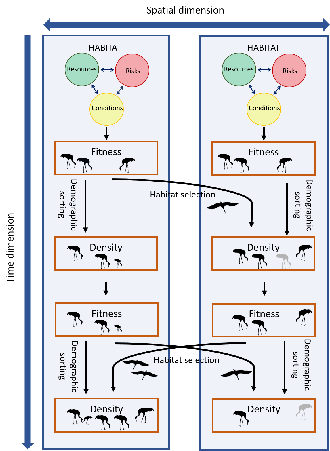
Figure 1.2: Fitness is the evolutionary currency determining an individual’s ability to transfer its genes to future generations. Individuals may be able to improve their fitness via plastic adaptations in physiology or behavior, for example by relocating and selecting more suitable habitats elsewhere. However, eventually they will have to face the demographic consequences of the environment they are exposed to. Their vital rates; births (depicted by small juvenile cranes) and deaths (depicted by gray cranes), will vary between habitats, and together with the redistribution of individuals, this demographic sorting will drive the spatial distribution and abundance of species.
First, there are associations between habitat and fitness. Here we define habitat-associated fitness as the contribution of each unit of habitat, \(\mathbf x\), to the population’s long-term log-rate of change (referred to as partial fitness in Jason Matthiopoulos et al., 2015). Partial fitness can be interpreted as the fitness of a population living in an environment made up entirely of habitat type \(\mathbf x\). The mechanisms underpinning the association between habitat and fitness are often sub-organismal, operating at the level of physiological capabilities, anatomy and life history strategies. We can often measure these fitness relationships with carefully constructed experiments or field observations. For example, fundamental biology of resource uptake or temperature tolerance in plants may be experimentally measured in the lab, metabolic costs can be gleaned from thermodynamic first principles, or for animals in the wild, accelerometers can be used to measure energetic costs or gains (Wilson et al., 2020). For example, changes in elephant seal body fat may be inferred from changes in sink-rate during drift dives, occurring in different habitats (Bailleul et al., 2007). Habitats that make a low contribution to fitness may ultimately lead to a loss of condition and subsequent demographic costs.
Second, we see associations between habitat and changes in species-density. Many organisms can mitigate the consequences of fitness, for example through their patterns of growth, defense activation and even whole body-metamorphosis. However, when organisms living in specific habitats experience low fitness, they either have to relocate or face the demographic consequences, like mortality and loss of reproductive potential. These processes will manifest themselves as changes in species density. The dynamical processes of relocation involves movement of individual animals, groups, or entire populations. The patterns in these movement trajectories can inform us about how the animal responds to its environment. For example, movement trajectories that look localized and sinuous are likely to be occurring in regions of high resource availability, or at least regions that appear worth exploring for resources. For organisms that cannot relocate, their density will ultimately be affected by habitat-mediated survival and reproduction. These vital rates define the intrinsic growth rate of a population and relate to the fundamental niche of a species (Holt, 2009).
Third, there are associations between habitat and species-density. The existence of an organism somewhere is mediated by fitness and dynamics in a series of complex causal steps. The emerging species distribution patterns are arguably the easiest to observe directly, in the wild, and are therefore the easiest to construct empirical models for (collectively called Species Distribution Models (SDMs)). While spatial variations in density may not reflect mechanisms operating at the immediate short term (e.g. days, hours or minutes), the spatial density of a species reflects accumulated effects of processes operating over longer time scales (e.g. years or multiple generations) and may ultimately be more informative about the place and role of that species in the earth’s biosphere.
In summary, phrased in more traditional terminology, associations with fitness define the fundamental niche of a species. The realized niche is represented by the eventual mapping of the distribution of a species in geographical space. In-between those two, we have a wealth of dynamics, represented by the associations between habitat and mechanisms of change. So, while species distribution is often implicitly assumed to be proportionally (or, at least, monotonically) linked with fitness, this is only the case in special circumstances.
1.5 What mechanisms drive habitat-mediated changes in species densities?
The underlying, and often unseen, forces shaping fitness manifest themselves in the distribution of a species via different dynamic mechanisms. Here, we make the important distinction between selective use of habitats at the individual level and demographic forces at the population level.
1.5.1 Behavioural selection
Basic patterns of behavior can be assigned to all organisms. For example, some plants may be triggered to release seeds only under certain conditions and propagule dispersal may be allowed to continue until suitable settlement conditions have been met (Grohmann, Hartmann, Kovalev, & Gorb, 2019; Seale et al., 2019). However, behavioral selection is most clearly seen in organisms that can perceive multiple stimuli from their environment and have control over their mobility. For some organisms, voluntary mobility may happen only once during a specific life-stage. For example, most bivalve species have a pelagic, long-ranging, larval stage, but once they settle, they may remain sessile for the rest of their lives. Most herbivores and their predators, however, may move great distances during their lives and continuously select habitats that fit their needs.

Figure 1.3: Plant species, like the dandelion (Taraxacum officinale) can regulate their dispersal and soil attachment in response to environmental conditions, like moisture and soil structure (Grohmann et al., 2019; Seale et al., 2019). Photo credit: Half-Seeded Dandelion by Wonglijie – CC BY-SA 3.0.
The process of voluntary movement comprises two different decision processes, each with different determinants and cognitive requirements. First, a decision must be made on whether to stay or leave, and second, a decision is needed on where to go. These decisions may happen simultaneously, sequentially or iteratively. Decisions on leaving are closely linked to patch departure rules or giving-up times (Charnov, 1976; Joel S. Brown, 1988). For example, one well-known theoretical approach to optimal decisions for patchy resources is the marginal value theorem which posits that once an individual depletes resources locally to a point that its intake rate drops below the average long-term intake rate, it should leave the patch (Charnov, 1976). However, since the actual or perceived long-term intake rate may gradually change over time (e.g. due to environmental change or learning abilities) and because animals often cannot instantaneously determine what local intake rate is (e.g. due to the stochastic nature of resources), they have to learn (Ollason, 1980). Several models are possible for the process of learning, even ones using direct metaphors from statistical laws, such as Bayesian updating of experience (Biernaskie, Walker, & Gegear, 2009). Learning takes time and may lead to sub-optimal decisions and a miss-match between the distribution of resources and species distributions, particularly if the environment is unpredictable (Kamil, Misthal, & Stephens, 1993; Riotte-Lambert & Matthiopoulos, 2019).
Having decided to leave, animals may then move randomly (e.g. following isotropic or correlated random walks) or exhibit directed movement based on their sensory perception, spatial memory or information from conspecifics (Fagan et al., 2013; Bracis & Mueller, 2017; Jesmer et al., 2018). While these well-recognized behavioral processes are of vital importance, they have only recently been explicitly included in SHA models (Oliveira-Santos, Forester, Piovezan, Tomas, & Fernandez, 2016; Merkle et al., 2019). For example, use-versus-availability analyses (see Chapter 2) compare used habitats to those habitats available within a next movement step (e.g. Step-Selection Functions) or within their home-range (e.g. Resource-Selection Functions). But, what about habitats beyond this range - do individuals perceive and avoid them? It is clear that realistic SHA models need to consider that individuals integrate information over much larger time intervals than the arbitrary scale of data collection. Cognitive processes can operate at several scales, some very small, others very large, and none of them need be similar or biologically relevant to the scale used in the data collection and subsequent analysis. If we are to understand SHAs, it is important to recognize the underlying mechanisms shaping individual movements and find a way to include these (or include emergent, accessibility constraints that are derived from these mechanisms) into our empirical models.
1.5.2 Demographic sorting
While the fine-scale distribution of organisms, such as animals, that can move in a voluntary and controlled fashion will be strongly shaped by behavioral selection processes, the distribution of all organisms will be shaped by demographic processes that are highly dependent on spatially heterogeneous environmental variables. Demographic sorting is particularly relevant for plants. Following an initial period of dispersal, which could be highly localized (e.g. via stolons) or wide-ranging (e.g. wind or animal dispersal), most plant propagules will become sessile. From that point onward, demographic processes determine whether a seedling will manage to germinate and survive. This combination of dispersal and habitat-driven demographic sorting can cause intergenerational movement across the landscape (see Fig. 1.4).
Similar demographic processes shape mobile animal distributions, but the combined action of demography and mobility makes their relative contributions difficult to tease apart. For example, when we fix an observation device (e.g. a GPS logger) onto a mammal, our view of the individual’s lifetime performance is truncated to the time-window of observation and all our inferences are conditional on the animal being alive and present at the original capture location. Demographic sorting has taken place prior to tagging, and clearly we can only study the behavioral selection of those individuals that managed to stay alive.
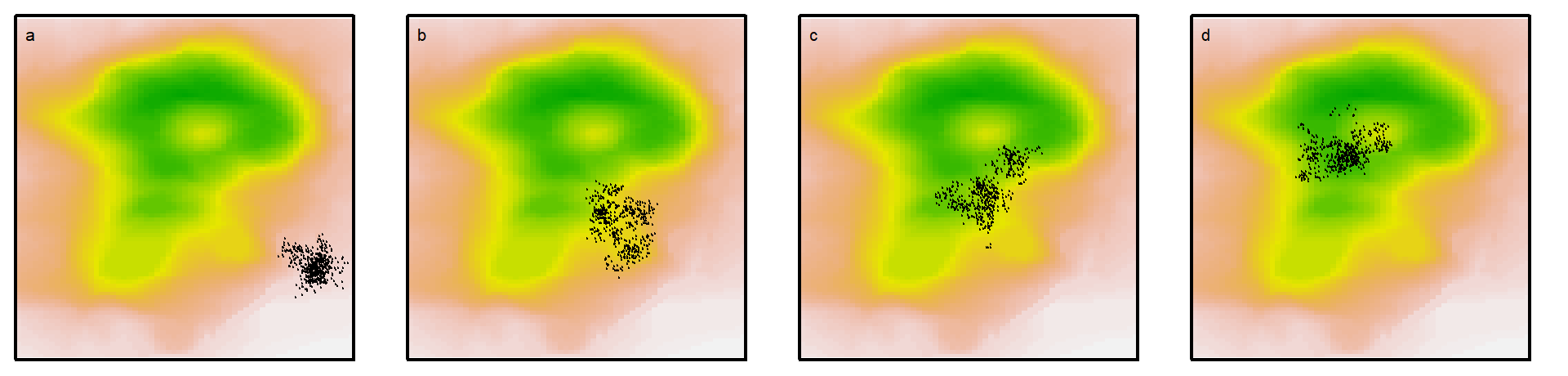
Figure 1.4: Inter-generational movement of members of a sessile species (e.g. a plant) progressing directionally through a combination of non-directional dispersal and demographic sorting. Suitable habitats are in shades of green, sub-optimal ones in yellow-to-brown. If we examine plant distributions over longer (multi-generational) time-scales, such that demographic selection is considered instantaneous, they display high mobility and dynamics. At these scales, patterns of selectivity may be reminiscent of animal redistribution.
1.6 When is species density a reliable reflection of habitat suitability?
When we observe a species at high density, we often make the implicit assumption that the local habitat must be good for the species, i.e. the intrinsic fitness contributed by the habitat (\(F_\mathbf x\)) is high, but this assumption is not necessarily valid. Below, we outline assumptions necessary for the distribution of a species to be proportional to fitness. Since the transition between fitness and species distribution can be driven by habitat-driven demographics and behavioral selection, we will formalize the link between fitness and distribution for these two avenues separately using a null model.
1.6.1 Why do we need a null model for SHA?
Each species will most likely be unique with respect to its relationship with its environment, and therefore it is tempting to develop SHA models in isolation. However, achieving some unification and contributing towards broader ecological theories is desirable, and this calls for a null model of species-habitat associations. Good null models can be useful for making sense of the world quantitatively, and they form the basis for further model development, as the initial assumptions become increasingly relaxed. These two properties of utility and expandability can stimulate scientific thinking and make null models good platforms for development. However, it is important to guard against over-interpreting null models in the face of data (this often happens when we inadvertently forget about their underlying assumptions).
A null model is a mathematical construct, derived from a set of assumptions that form the basis for discussion on a physical process. In the development of null models, mathematical convenience is prioritized over the realism of the assumptions, to ensure that the basic results can be derived analytically and exactly. For example, in physics, an ideal gas is a hypothetical form of matter that comprises dimensionless and massless molecules, that are unaffected by forces other than those resulting from perfectly elastic collisions between them. Despite these patently unrealistic assumptions, the null model of ideal gasses has led to invaluable and approximately applicable rules in thermodynamics. In economics, the null model of supply and demand has been used successfully to understand price determination for goods and services. Its key simplifying assumption is that it considers omniscient and logical consumers who focus exclusively on a particular commodity, while keeping their behavior constant with regard to other goods. The model has been so successful among economists, despite these assumptions, that people are occasionally (and unfairly) surprised when its predictions diverge from reality.
Ecology has its fair share of null models. Examples include the logistic model in population dynamics (Verhulst, 1845; Pearl & Reed, 1920), the model of perfect mixing in predator-prey ecology and epidemiology (Law et al., 2008), the marginal value theorem in foraging ecology (Charnov, 1976), and the neutral theory of biodiversity (Hubbell, 2001). In the early stages of structuring this book, it occurred to us that for SHA, the research community has been implicitly using a null model, without specifying its mathematical formulation or explicitly stating its assumptions. This implicit null-model is essentially one that gives rise to a “pseudo-equilibrium assumption”, meaning that species respond to measured habitat covariates with no delay, and that species density is proportional to species fitness.
Species fitness, dynamics and population distribution, the three aspects of species that respond to habitat, are connected. Fitness affects dynamics, which affects distribution. In turn, distribution (through density dependent processes) affects habitat and fitness (Fig. 1.5). Below, we will formalize the link between fitness, dynamics and distribution, and we will try to connect our SHA null model with many of the already existing ecological null models. In the process, we will make sure that the null model has the two valuable properties of utility and expandability.
In Section (1.5) we have identified two mechanisms that determine SHA: Demographic sorting and behavioral selection. Below we will first develop a null model for each mechanism independently, and subsequently show how these two null models converge.
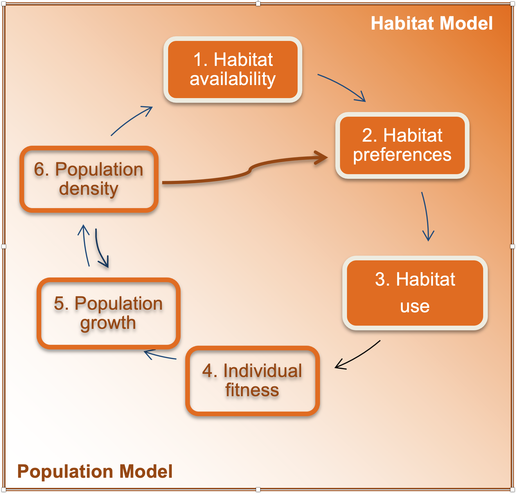
Figure 1.5: The chain highlighting how species fitness, dynamics and population distribution interact with habitat (modified from Jason Matthiopoulos, Field, & MacLeod, 2019). A region in space is characterized by the availability and spatial configuration of different habitat types (step 1). Organisms may actively or passively select specific habitats (step 2) which may lead them to use habitats disproportionately to their availability. Habitat availability and habitat selection give rise to the observed spatial distribution (step 3). The exposure of individuals to different habitat types will influence their fitness (step 4), which determines the collective capability of a population to grow (step 5). Processes of population change determine current population density (step 6), which has the opportunity to alter habitat availability and feed back directly into habitat selection and population growth via density dependent and spatial crowding.
1.6.2 A null model for habitat-driven demographic sorting
Let us imagine an ideal life-history organism with the following properties:
- It has a highly mobile dispersal stage, so that all of space is equally accessible to all of its propagules.
- It has a completely sessile reproductive stage, so that local density results from local habitat quality.
- Its intrinsic population growth is solely driven by habitat, and it is positive everywhere in the landscape.
- Its local population growth decreases linearly with local density.
- It has no other species to compete with.
For a given spatial location, \(\mathbf{s}\), with a particular set of environmental characteristics, \(\mathbf{x}\), we can model growth of local population density, \(N_\mathbf s\), in discrete time as
\[\begin{equation} N_{\mathbf s,t+1}=N_{\mathbf s,t}\exp(F(\mathbf x, N_{\mathbf s,t})) \tag{1.1} \end{equation}\]
The function \(F\) has two convenient names: growth rate and fitness. In classic population ecology, the population’s growth rate between two successive measurements is defined as \(\log(N_{t+1}/N_t)\). The population growth rate is equivalently called the fitness of a population (Nur, 1987; Jason Matthiopoulos et al., 2015). So, let us consider the local growth rate of a population as a trade-off between the intrinsic fitness value of the habitat (i.e. \(F(\mathbf x, N_t\approx0)= F_0(\mathbf x)\)) and the attrition \(b\) inflicted onto population growth (i.e. onto population fitness) by the addition of a single individual:
\[\begin{equation} F(\mathbf x, N_{\mathbf s,t})=F_0(\mathbf x) -bN_{\mathbf s,t} \tag{1.2} \end{equation}\]
From equations (1.2) and (1.1), we get the model
\[\begin{equation} N_{\mathbf s,t+1}=N_{\mathbf s,t}\exp(F_0(\mathbf x) -bN_{\mathbf s,t}) \tag{1.3} \end{equation}\]
We can now look at the two extremes of population density. At one extreme, when the population density is very small (i.e. \(N_t\approx0\)), its growth rate is equal to the intrinsic growth rate \(F_0(\mathbf x)\). At the other extreme, when the species has sufficient time to reach an equilibrium local population density (i.e. \(N_{\mathbf s,t+1}=N_{\mathbf s,t}=N_{\mathbf s}^*\)):
\[\begin{equation} N_{\mathbf s}^*=F_0(\mathbf x)/b \tag{1.4} \end{equation}\]
In biological terms, attrition caused by density dependence has annulled the benefits of habitat, and the equilibrium distribution becomes proportional to the intrinsic growth rate. In Fig. 1.6 we try to visualize how, for a growing population of ideal life-history organisms, the equilibrium density in each cell eventually becomes proportional to \(F_0(\mathbf x)\).
Because our ideal organisms behave as a closed population within each location, the SHA null model can be linked to the null model used in single-species population dynamics, the logistic equation1
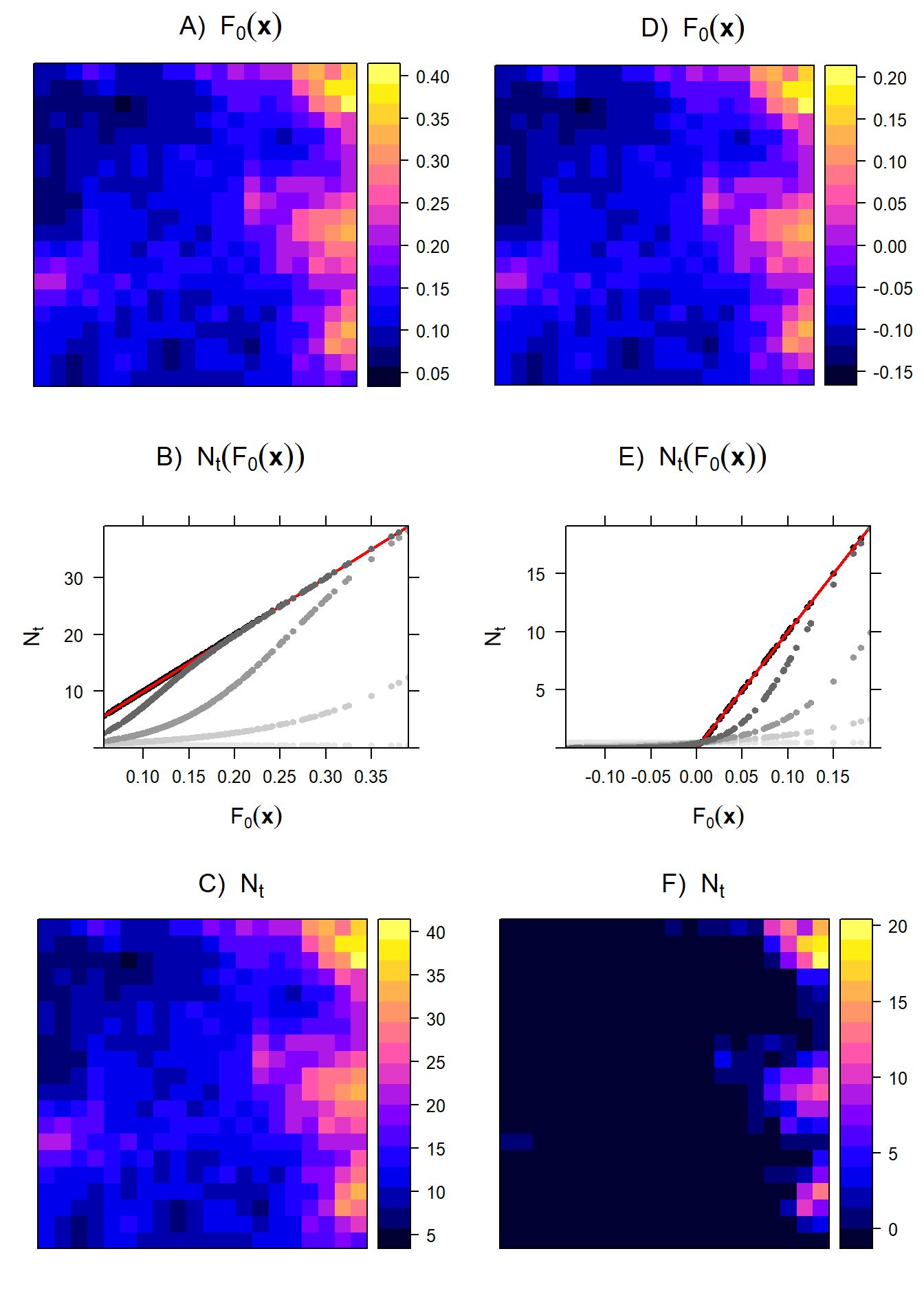
Figure 1.6: Simulation of an ideal life-history organism: We set out to visualize the relationship between fitness and distribution during the growth of a population from \(N_{\mathbf s,t=0}\approx0\) to the local equilibrium density \(N_{\mathbf s}^*\). The experienced fitness \(F_\mathbf x\) at low population size is defined as a linear function of a covariate \(X\) representing food. We explore two scenarios, one where \(F_\mathbf x\) is always positive across space (A) and one where \(F_\mathbf x\) can also be negative in some areas of space (D), achieved by subtracting a constant value from the original non-negative \(F_\mathbf x\). The population growth rate is defined as \(N_{\mathbf s,t+1}=N_{\mathbf s,t}\exp(F_\mathbf x -bN_{\mathbf s,t})\) where b=0.01. The simulation is run for 250 years. At the start of the simulation (\(t=0\)), the local population size \(N_{\mathbf s}\) is still independent of \(F_\mathbf x\) (light gray points, in B). Ultimately, the relationship will equilibrate to a linear relationship between local carrying capacity \(N_{\mathbf s}^*\) and \(F_{\mathbf x}\) (black points in B), with slope coefficient of \(1/b=100\) (red line in B)). The same applies to the scenario where \(F_\mathbf x\) can also be negative, but this will result in truncation of \(N_{\mathbf s}^*=0\) when \(F_{\mathbf x}\le 0\) (E). Spatial maps of \(N_{\mathbf s}^*\) are shown in C and F. Note that when a landscape contains locations with negative fitness (i.e. \(F_{\mathbf x}\le 0\)), this will result in the emergence of a patchy distribution of a species (F).
1.6.3 A null model for habitat selection
We build upon the work of Fretwell & Lucas (1969) who consider the distribution of an ideal free species to be a purely behavioral phenomenon, with no demographic sorting involved.
The assumptions underlying the ideal free organism are:
- Individuals are aware of the current value of each patch2 and settle in the patch most suitable to them (i.e. individuals are ideal foragers).
- All individuals are free to enter any patch, and arriving individuals do not have a disadvantage compared to individuals that are already there, all individuals are genetically alike or of the same phenotype, and all patches are equally and instantaneously accessible to all members of the species.
Now let us consider the behavioral mechanism that shapes the distribution of ideal-free foragers. The first individual will select a single patch \(i\) with the highest baseline suitability \(B_i\), ignoring all other, lower-quality patches. By making use of the patch, the patch baseline suitability \(B_i\) will be reduced to a lower suitability \(S_i\). The next individual that comes along, will select a patch with the highest suitability \(S\), which could be the same patch \(i\) or a different one. This process is repeated for all individuals in the population (see also Fig. 1.7). Eventually this process results in a landscape where all \(l\) occupied patches have equal suitability; \(S_1=S_2=...=S_l\). The formula quantifying how \(S_i\) depends on the baseline suitability \(B_i\) and species density \(N_i\) is:
\[\begin{equation} S_i=B_i-f(N_i),\ i=1,2,...N \tag{1.5} \end{equation}\]
Fretwell & Lucas (1969) treated habitats as discrete patches. For a given spatial location, \(\mathbf{s}\), with a particular set of environmental characteristics, \(\mathbf{x}\), the continuous formulation for eq. (1.5) is:
\[\begin{equation} S(\mathbf x, N_{\mathbf s,t}) = B_\mathbf x -f(N_{\mathbf s,t}) \tag{1.6} \end{equation}\]
Since natural selection leads to the evolution of behavior, the perception of habitat suitability by perfectly adapted individuals should correspond to the fitness value of those habitats (see also assumption 1). In that case, the baseline suitability, \(B_i\), corresponds to the intrinsic population growth rate at low population density (\(F_{\mathbf x}\)), and the emerging suitability in the presence of conspecifics, \(S_i\), will be equivalent to \(F(\mathbf x,N_t)\). In that case, eq. (1.6) becomes:
\[\begin{equation} F(\mathbf x, N_{\mathbf s,t})=F_0(\mathbf x) -f(N_{\mathbf s,t}) \tag{1.7} \end{equation}\]
Unlike us, Fretwell & Lucas (1969) were not explicit about the functional form or mechanism underlying \(f(N_i)\), but two possible mechanisms that can lead to eq. (1.5) are interference competition and explorative or scramble competition (Křivan et al., 2008). Given these assumptions, Fretwell & Lucas (1969) showed that, for each positive total population size \(M\), there will be a unique Ideal Free Distribution (IFD) (see also Fig. 1.7). Now, let us consider the special case where fitness declines linearly with local population density (i.e. \(f(N_{\mathbf s,t})=bN_{\mathbf s,t}\)), and where the total population size \(M\) is at carrying capacity, such that, \(F(\mathbf x, N_{\mathbf s}^*)=0\) everywhere within the study region:
\[\begin{equation} F(\mathbf x, N_{\mathbf s}^*)=F_0(\mathbf x) -bN_{\mathbf s}^*=0 \tag{1.8} \end{equation}\]
which implies
\[\begin{equation} N_{\mathbf s}^*=F_0(\mathbf x)/b \tag{1.9} \end{equation}\]
In summary, when total population size of ideal free foragers is at carrying capacity, the relationship between density and habitat suitability or fitness (eq. (1.9)) is identical to that for the ideal life history organism (eq. (1.4)).
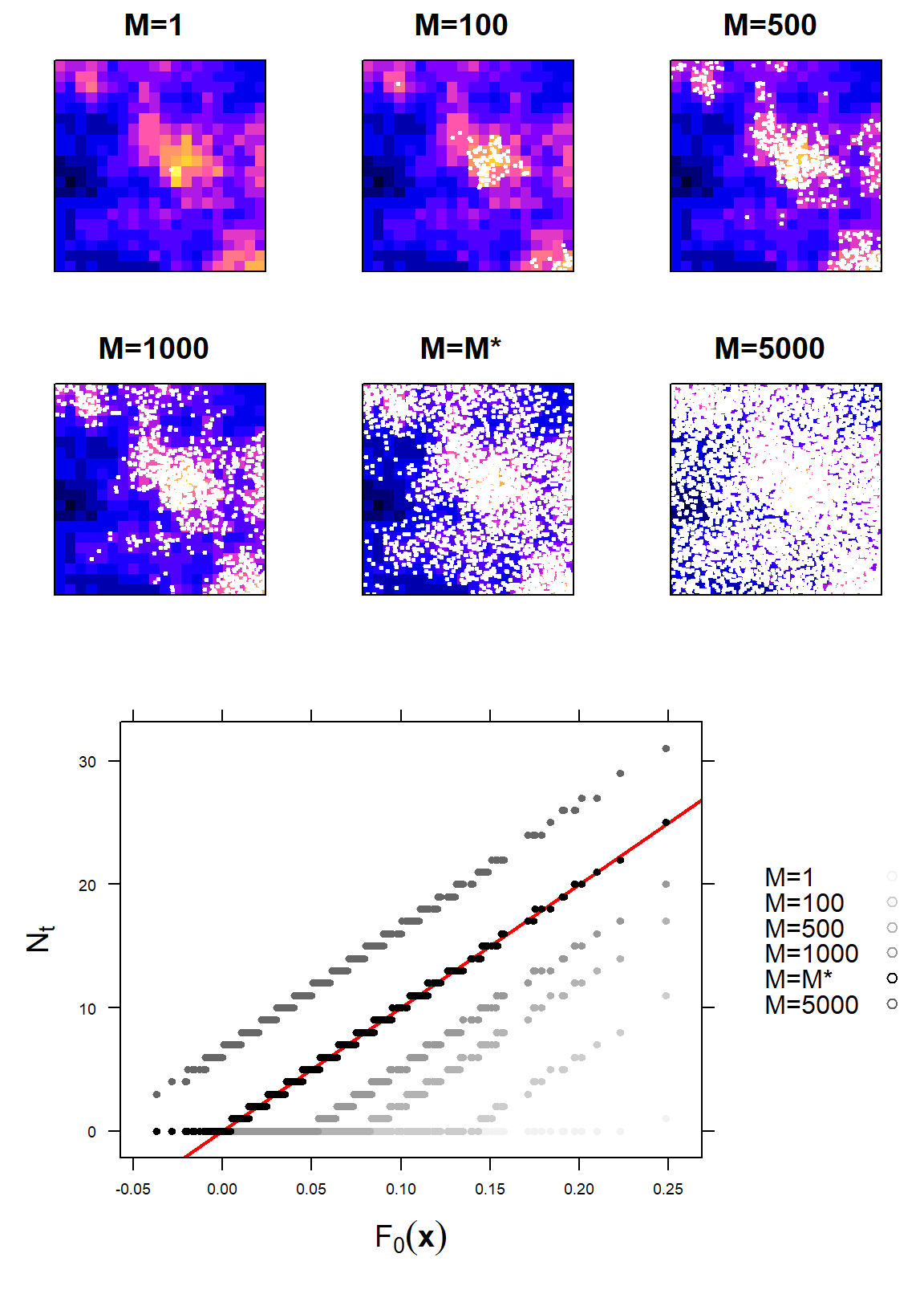
Figure 1.7: The relationship between the baseline suitability (\(B_i\) in Fretwell & Lucas, 1969) or intrinsic fitness \(F_0(\mathbf x)\), and local density (\(N_{\mathbf s}\)), shown for an increasing total population size (\(M\)) of ideal-free organisms (as proposed by Fretwell & Lucas, 1969). The top figures show habitat suitability represented by intrinsic fitness. The white dots represent the distribution of individual animals for different total population sizes (\(M\)). In the bottom figure, the different shades of gray represent the different population sizes (\(M=1,50,100,500,1000,5000\)), with light gray for \(M=1\) and dark gray for \(M=5000\). Black dots and red line show the relationship between \(N_{\mathbf s}\) and \(F_0(\mathbf x)\) when the population is at carrying capacity, i.e. \(F(\mathbf x, N_{\mathbf s,t}) = 0\). Individuals always select the habitats with the highest current \(F(\mathbf x, N_{\mathbf s,t})\). When habitat quality diminishes as a linear function of local population density, this will result in a linear relationship between baseline habitat quality \(F_0(\mathbf x)\) and the observed species density \(N_{\mathbf s}\) for all occupied locations, and \(N_{\mathbf s}=0\) for all other locations.
1.6.4 Is population size or population growth a better proxy for fitness?
Our identical null models (eq. (1.9) and eq. (1.4)) hint at the fact that equilibrium population size and intrinsic growth rate could both provide valuable clues about the underlying fitness contributed by habitats. Historically, the niche literature has focused on the ability of a population to grow (Holt, 2009) and the species distribution literature has focused on pseudo-equilibria (Guisan, Thuiller, & Zimmermann, 2017), but the intuitive notion is shared. Whether we are talking about fitness in niche space or habitat suitability in geographical space, we want to get a handle on which habitats are “good” and “bad” for an organism.
So, looking ahead at the types of data that we should be collecting and analyzing, does the null model offer any insights into whether data on intrinsic growth or equilibrium distribution is more useful? The short answer is that both have limitations and, ultimately, data on both may be required. A longer answer goes as follows: Data on intrinsic growth rates are difficult to collect. They require us to observe a local population at a small enough size that density dependence is not affecting growth. Growing populations, by definition stay small only temporarily. Catching a species at such a transient state at sufficiently many habitats to enable a SHA model to be fitted is quite unlikely. Certainly, longer-lasting states (e.g. close to a stable equilibrium) are more amenable to observation. However, as the null model suggests, landscapes at-equilibrium yield leveling inferences for the poorest of habitats, because local populations observed in negative fitness habitats are always extinct in the long-term, so we have no way of learning about different shades of “bad habitats” (See also Fig. 1.6F)
The choice between intrinsic rates and equilibrium sizes becomes more tangled when one of the limiting resources driving fitness is depletable. The overall abundance and detailed spatial distribution of the resource will be different when the consumer is sparse compared to when it is at its carrying capacity. Which of those resource distributions is more relevant to a SHA model?
Consider the following thought experiment, whereby the intrinsic population growth rate is a function of current food availability. At the earliest stages of consumer growth (and resource depletion), a correlation between the distribution of food and consumer growth rates would deliver an informative SHA. Food-rich locations would give faster growing consumer populations. However, it is rarely the case that populations are captured at such initial stages of development, and it is unlikely that the initial development happens in a spatially synchronized manner (as opposed to a local invasion). If, on the other hand, we wait for the equilibrium distribution to develop, depletion distorts our inferences. As predicted by the IFD, the equilibrium density of the consumer will yield no relationship with food density, but a strong positive correlation with rate of food replenishment. Hence, correlating consumer density with standing crop may give us the misleading impression that the consumer is indifferent or even avoids its key resource. Using resource productivity data as a covariate would, of course, dispel this myth but such data are almost never available in the field.
Hence, in the case of depletable resources, it makes sense to relate resource growth to equilibrium consumer distribution, and it also makes sense to relate initial resource distributions to consumer intrinsic growth rate, but it is not meaningful to correlate simultaneous snapshots of the distribution of the study species and its resource. Given that data on distributions are much easier to collect than data on rates of change, we have a fundamental problem of indeterminacy in correlational models.
1.7 When are the null model assumptions violated?
The two null models for demographic sorting and behavioral selection, both describe the proportional relationship between habitat-specific intrinsic fitness and the species’ equilibrium density. There are two main reasons why this proportionality assumption is violated. First, the null models might be inappropriate. For example, the models assumed that an increase in species-density led to a proportional decrease in habitat quality and associated fitness. In many systems, changes in species density might have a non-linear effect on habitat-associated fitness. Second, the transition towards the equilibrium density takes time. In fact, constraints in species demography and mobility, in conjunction with changing environments, might mean this equilibrium distribution is never reached. However, being able to consider a snapshot of a species distribution as a static reflection of underlying habitat suitability (the pseudo-equilibrium assumption) is certainly convenient and our null model allows us to think in these terms. Yet, it is important to remember just how restrictive a set of assumptions we needed to make for the pseudo-equilibrium assumption to hold. We take some time in this section to examine the ways in which the real world can violate the assumptions of our null models. These violations will prompt improvements to the basic SHA framework in later chapters of this book.
1.7.1 When the relation between species density and fitness is non-linear
Our null model assumed that species density responds continuously to fitness and that fitness is non-negative throughout the landscape. However, population density does not always scale linearly with fitness. For example, nesting seabirds establishing at suitable locations exclude their competitors and form equally spaced nesting arrangements. Almost undoubtedly, some nesting locations are more suitable than others, but as long as the suitability of a nesting site is above a nominal threshold, it will eventually be occupied. Once occupied, no additional breeding pair can settle on that location. Our observations at equilibrium will therefore only be able to capture a binary state of occupancy/vacancy, rather than a continuous measure of suitability.
The effect of species density on fitness can also be positive. For example, many species aggregate to create positive feedbacks between group members, to reduce predation risk, modify their the environment, and exchange information and services. These are also known as Allee effects (Allee, 1951; Stephens & Sutherland, 1999). For example, social species, like cetacean, operate in groups to improve the detection and exploitation of fish schools. As a result, even habitats with negative intrinsic fitness may generate positive fitness once the density of cooperating individuals increases (Fig. 1.8). As a result, the relationship between density and intrinsic fitness may be non-linear at low population densities.
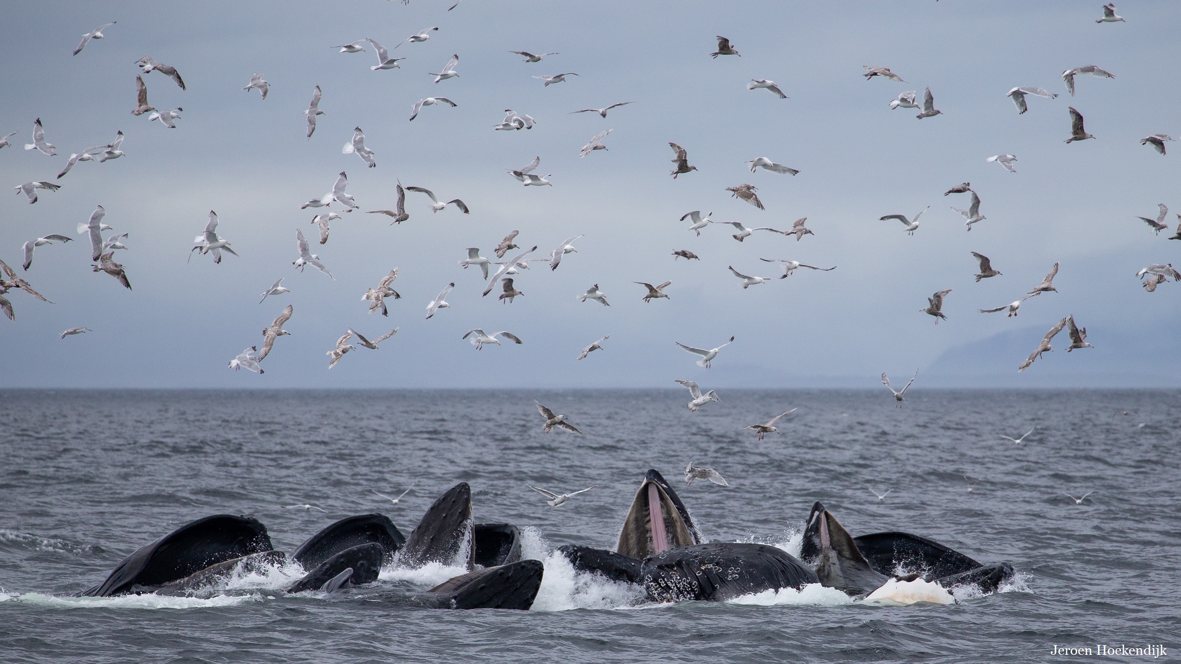
Figure 1.8: Collective feeding by Humpback whales (Megaptera novaeangliae) in Alaska (USA). The null models for demographic sorting and behavioral selection assume that habitat quality declines linearly with the increase in species-density. For most social, cooperative organisms this linear relationship does not hold; fitness may increase as function of group size (the Allee effect), which results in a non-linear relationship between fitness and population densities. Photo: Jeroen Hoekendijk.
1.7.2 When species occur at places with negative fitness
Organisms are often encountered in poor-quality habitats. Most obviously, this can be a transient state; Organisms move at finite speed and may cross hostile or barren habitat while moving in-between good-quality habitats that are within reach (Jason Matthiopoulos, Fieberg, Aarts, Barraquand, & Kendall, 2020). Organisms may also be pushed into suboptimal habitats more permanently, creating extinction debts: Temporal lags in the decline of a population may leave remnants in poor quality habitats and give misleading results if we incorrectly assume pseudo-equilibrium states.
Less intuitive, however, is that mobile organisms may actively choose to spend time in habitats of negative fitness. Indeed, viable animal populations may be observed in landscapes where no single point is characterized by positive fitness; the zero niche paradox (Fig. 1.9). This possibility occurs because, while immobile organisms must match themselves to their environment, mobile organisms have the ability to match their environments to themselves (Begon, Harper, & Townsend, 1996). By moving around, mobile organisms can accumulate resources, reduce risk and mitigate environmental conditions to ensure fitness is positive overall. Sometimes, all necessary environmental conditions and resources are in relatively close proximity, which allows animals to live in a relatively compact home-range. However, for other species, like many migratory animals, the required resources/conditions might be transient, or separated by thousands of kilometers, requiring long-range movements. In general, whether a fitness integration is determined by the spacing between different habitats and the mobility of the animals that exploit them.
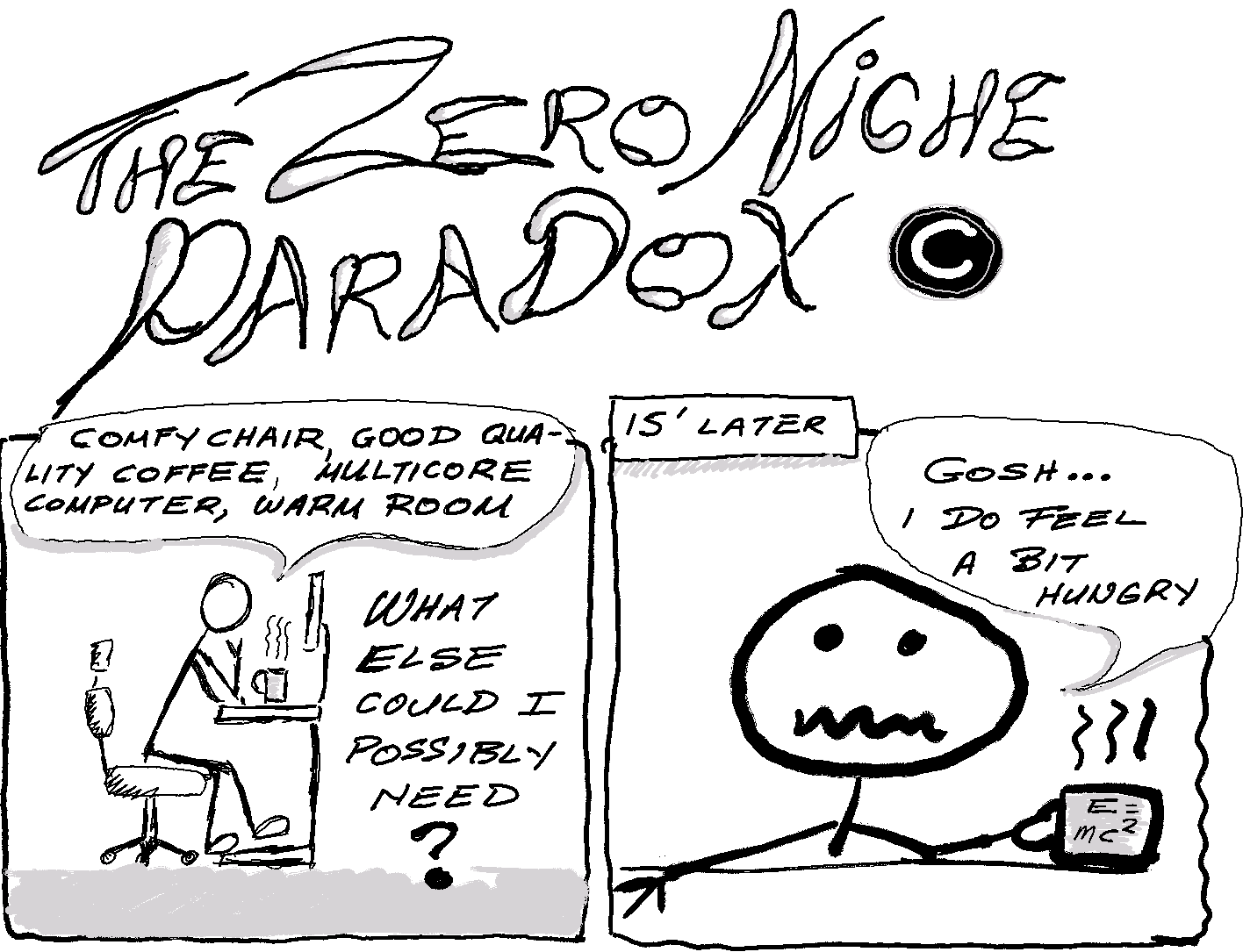
Figure 1.9: No matter how suitable a habitat is for our survival at any given time, it is often necessary to use several habitats in combination to achieve positive fitness. At a fine enough spatial and temporal scale, it is conceivable that no single habitat can offer positive fitness. Ostensibly, that is the reason animals move in space and plants do different things at different times of the year.
Fitness integration may also be possible for sessile organisms that may be able to exploit temporal (i.e. diurnal, or seasonal) transitions in the resources and conditions available at their fixed locations. For example, plants may regulate their tolerances so that they can withstand temporal separation between peaks of availability in the same, or complementary resources. The notion of temporal proximity of vital environmental circumstances is another manifestation of the problem of accessibility (introduced above in the context of space, and mobile organisms) that is not readily visible by simply mapping fitness in environmental space.
1.7.3 When species do not occur at places of positive fitness
Just as organisms may be found at places of negative fitness, they may be absent from areas of positive fitness. In conservation ecology this is known as a ‘colonization credit’ (Watts et al., 2020), a result of the fact that it may take time for individuals, populations and species to respond to changing environments. Environments can be highly dynamic. Mismatches between high habitat suitability and the abundance of a species may arise from imperfect knowledge of the landscape or limited relocation speed. A resource, like the massive release of eggs by spawning fish (Ims, 1990; Šmejkal et al., 2018), may suddenly become available and it may take some time before a forager can locate and exploit it. Sometimes, environmental changes are unpredictable and the ability of organisms to benefit from them is limited by their range of perception. The pressure to quickly and accurately assess the availability of resources has selected for sophisticated visual, auditory, gustatory, olfactory and somatosensory capabilities. However, the ultimate extensions to perception come from higher cognitive functions, such as memory and communication, which are extremely useful for exploiting both predictable (e.g. seasonal) or unpredictable habitats. For example, memory may allow an individual to relocate in anticipation of the appearance of resources, suitable conditions or the departure of predators. For example, many migratory birds start their journey in anticipation of high resource availability elsewhere and start breeding well before the peak in insect abundance.
Absence of a species from apparently suitable habitat may be caused by medium-term delays, covering the life span of individuals. Most organisms have distinct life stages, each potentially characterized by different mobility, resource requirements and sensitivity to environmental conditions. For example, jellyfish have a distinct and sessile polyp phase and a free-moving medusa phase. Insects, like butterflies, have well-defined larval and adult stages. Even the types of risk that individuals are vulnerable to can change as they metamorphose or grow. The habitat requirements of distinct life-stages may be dramatically different and, even, mutually exclusive. If the habitats needed for different life-stages are not sufficiently close to each other, then the organism will occur in none of them. This suggests that the mobility of different life stages must be understood in a habitat context. For example, many fish species have very specific spawning areas, from which free-floating fertilized eggs, or larvae, are transported by the currents towards nursery areas. It also underlines that successful SHA models must consider how mobility constraints operate across an individual life history.
At longer time scales, delays can occur trans-generationally as a result of transient population dynamics, particularly if the landscape is changing continuously. Colonization and invasion processes may take many years even for the most advanced and mobile of animals (see Grey whale example, Fig. 1.1). Conceivably, trans-generational delays are the result of cultural behavior in animals with high levels of cognition (Jason Matthiopoulos, Harwood, & Thomas, 2005). Grey seals had been absent from the Wadden Sea since the middle ages, despite there being suitable habitat, and the presence of nearby gray seals around the UK coastline. Once a breeding population established in the Wadden Sea, the population quickly grew (Brasseur et al., 2015).
Ecological dynamics beyond single-species growth becomes an even more severe complication to the null model notions about SHA. In natural systems, multiple species interact, either directly or indirectly. If the effects can be considered unidirectional, then the focal species can be regarded from a Hutchinsonian viewpoint (Hutchinson, 1957) by including all other influential species (e.g. prey, predators) as resource or risk dimensions of the environmental space. However, if interactions are fully bi-directional, then we need to take an Eltonian viewpoint (Soberón, 2007) to acknowledge that a species responds to the environment, but also influences the availability and behavior of properties of its environment. We have already discussed how consumer resource dynamics can complicate our inferences. Although we looked solely at the mechanism of depletion, predators may also impact the distribution of a mobile prey through indirect mechanisms such as landscapes of fear. Other mechanisms of environmental alteration without direct depletion include various forms of ecosystem engineering (Odling-Smee et al., 2013) and indirect community effects. For example, tree shadows reduce wind below the canopy and increase ambient humidity. Blue mussels (Mytilus edulis) attach themselves to each other and collectively create a structure that is less susceptible to environmental stress, like waves and currents, and can house a multitude of other organisms (Fig. 1.10). There are currently few attempts to fit dynamical, multi-species SHA models to field data (but see Ovaskainen & Abrego, 2020), a task that seems as intimidating as it is worthwhile.
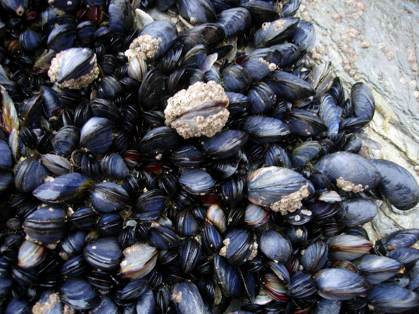
Figure 1.10: The blue mussel (Mytilus edulis) is an important ecosystem engineer in coastal intertidal and subtidal ecosystems. Its association with its environment is bi-directional; Its presence can strongly alter the type of habitat, influencing the presence of other species. An Eltonian viewpoint is required to quantify their habitat association. Photo credit: Cornish Mussels by Mark A. Wilson – Public Domain.
Most of the above obstacles leading to an absence of the focal species from apparently suitable habitat are overcome by plastic (e.g. behavioral) responses of individuals or numerical responses of populations. Evolutionary responses may also occur at the species level and at potentially slower rates, although sometimes rapid selection occurs on time-scales similar to population dynamics (Bassar et al., 2010). Hence, a portion of the species may be able to live in a new region outside the current species range, but they may have yet to reach it. This discussion highlights the possibility that species tolerances are fluid, and hence that SHAs are non-stationary due to rapid evolution. Evolution would violate the assumptions of even the most sophisticated statistical SHA models, but is currently low on the wish-list of extensions.
1.8 The SHA models we wish for and the SHA models we have
Our proposed null model in section 1.6.2 may be new, but it spells out the implicit assumptions of nearly all SHA models in existence today. Their key desire is to assume that the study species is found at all suitable places and is absent from all unsuitable places (Guisan & Thuiller, 2005; Gallien et al., 2012). This is known as the pseudo-equilibrium assumption. But why the prefix “pseudo”? Because every ecologist is fully aware of the mechanisms that can violate our null model assumptions. For instance, every ecologist can recognize that species abundance may be capped above or below so that it is not consistently indicative of habitat suitability gradients. Species can survive indefinitely in areas of negative fitness by using habitats in a complementary way or by buffering against brief periods of adversity. Species may be observed temporarily in completely unsuitable areas due to extinction debts, but conversely, they may be absent from areas of positive fitness because of colonization credits.
The raison d’etre for the pseudo-equilibrium assumption (and, by implication, our null models) is that we wish to draw statistical inferences about fitness, suitability, viability and fundamental niches, but, instead, we have data on occurrence from museum records, line- or point-transect detections, individual telemetry tracking and spatial mark-recaptures. The type of SHA model that has so far been used to achieve the transition from distribution to fitness (and back again) is the Species Distribution Model (SDM). Its fitness inferences are valid only as a manifestation of our null model and the highly restrictive assumptions that it entails. Nevertheless, the general category of SDMs is currently our only route to modeling SHAs and must therefore be seen as a precious foundation on which to build. What kind of research program does this suggest for the future? The process of extending the SDM to become a fully-fledged SHA model will entail first, a recognition of the difference between fitness and distribution, second, an enumeration of the mechanisms that make them different (the mechanisms that violate the assumptions of the null model) and, third, the addition of modeling features in-between the state variables of fitness and distribution, to correct for these violations. We have taken the first and second of these steps in this introductory chapter. The third step is more of a voyage, and will take the rest of this book, and beyond, to complete.
To close this chapter, we present a comprehensive synthesis of the current versions of SDM that are encountered in the literature. Bear with us while we first pretend that there are only pure-forms of SDMs (section 1.9), to help us define the distinct flavors. We will then go on to present the results of cross-fertilization between them (section 1.10).
1.9 A puritan taxonomy of SDMs
At first sight, the diversity of methods available for converting spatial data to prediction maps can seem overwhelming. However, there is an emerging hierarchy in the methodological literature that considerably simplifies our effort to outline recommendations for best practice (Fig. 1.11). We can present this as a succession of four branchings, leading up to our preferred approach of inhomogeneous point process models
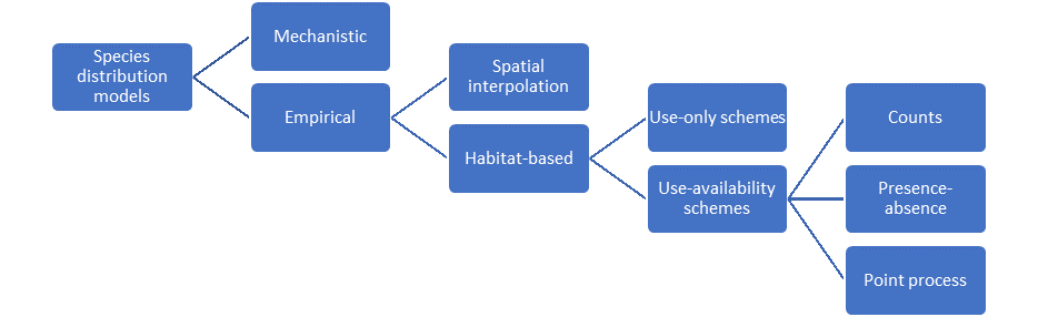
Figure 1.11: An overview of available methods for modeling species distributions leading up to our recommended approach.
Spatial predictions can be generated by building mechanistic models of animal movement and demography from first principles and scaling them up to population distributions (Paul R. Moorcroft, Lewis, & Crabtree, 1999, 2006; Paul R. Moorcroft & Barnett, 2008; Paul R. Moorcroft, 2012). Arguably, models with lots of biological detail (e.g. based on principles of physiological tolerance, movement behavior and social interactions) bring greater insights and predictive capability (Kearney & Porter, 2009; Hefley & Hooten, 2016). However, mechanistic modeling can be quite demanding technically and is generally more vulnerable to model misspecficification (models that disagree with the data) and parameter identifiability issues (situations where the data are not sufficient to estimate all model parameters). These problems can only be revealed if models are confronted with data. For example, the series of papers by Lewis and Moorcroft cited above, which form the state-of-the-art in mechanistic distribution modeling, require specific assumptions about animal movement and rely on sufficiently mathematical users who can formulate and manipulate partial differential equation models. Alternatively, we may choose to employ empirical, statistical models (Guisan & Zimmermann, 2000; Guisan & Thuiller, 2005; Guisan et al., 2017). The deciding trade-off between mechanistic and empirical models is one of realism and predictive capacity against the ease of use and robustness to misspecification. In this book, we build up from the foundations of the empirical model, but all of its extensions strive to increase its mechanistic content.
Within the class of empirical models (see review by J. Matthiopoulos & Aarts (2007)), we can distinguish between models that merely reconstruct the spatial density of a population (such as kernel smoothing, additive smoothing, or geostatistical methods) and regression methods that rely on habitat information as explanatory variables. Spatial density estimation methods rely on geographical proximity and the existence of spatial autocorrelation (Levin, 1992) to interpolate between observation points and map density in unobserved space, or alternatively, to smooth a finite data set of synoptic observations into a population-level expectation of usage. Density estimation methods focus on removing spurious variability from the predictions, but aim to stay as close as possible to the observations. Therefore, their ability to describe the available data is often better than that of habitat models (Bahn & Mcgill, 2007). Habitat models, on the other hand, are not by default spatial, since they are fitted in environmental (or niche) space (Pearman, Guisan, Broennimann, & Randin, 2008). Consequently, the greater ability of habitat models to interpolate and extrapolate spatially relies on the quality and relevance of their underpinning covariates. The deciding trade-off between density estimation and habitat models is one of faithfulness to the particular distributional data collected and the ability to extend predictions beyond the spatial and temporal frame of data collection. We aspire to generality, so we build on the habitat model as a foundation, but later return to spatially explicit extensions.
Within the class of habitat models, we distinguish between two main categories. The first, are known as profile methods and they argue that knowledge of where, in niche space, a species occurs is sufficient to understand its fundamental niche and map its current and future distribution. Broadly, this category includes methods such as climate envelope models and the use of multivariate statistical methods such as principal component analysis (PCA) for the analysis of presence-only methods (reviewed in Pearce & Boyce, 2006). The alternative class of use-availability schemes either contain representative information on the distribution of organisms (i.e. presence and absence), or they supplement presence data with availability data, allowing the models to contrast the habitat choices that organisms made, with the options that they had available to choose from. The broad area of use-availability schemes includes the vast literature on resource-selection functions (Boyce & McDonald, 1999; Morris, Proffitt, & Blackburn, 2016) and maximum entropy approaches (Elith et al., 2011; Merow, Smith, & Silander, 2013). Profile methods have been critiqued extensively in the methodological literature (see Pearce & Boyce, 2006 for a review), and there is really no sound scientific reason for choosing to use a profile method.
The final decision stage is mostly perceptual, relating to how space is conceptualized for the purposes of modeling the data. For example, space may be thought of as a regular grid (e.g. comprising squares, or other regular forms of tessellation, such as hexagons - see Grecian et al., 2016). In that case, the spatial data take the form of counts and are modeled by appropriate probability models such as the Poisson. Alternatively, and more realistically, space may be thought of as continuous and different spatial locations may be characterized by whether a species was present or absent. In that case, spatially referenced data take the form of zeroes and ones and the most appropriate probability model is Bernoulli (Aarts, MacKenzie, McConnell, Fedak, & Matthiopoulos, 2008; Gelfand & Shirota, 2019; Gelfand, 2020). Yet another approach within the continuous space framework is to imagine that observations of organisms appear at random locations almost like pin-lights that blink in and out at different time frames of observation. This framework, known as the Inhomogeneous Point Process (IPP) models the occurrence of events within a unit of time and space as originating from a smooth intensity surface, describing the instantaneous and infinitesimal rate of the Poisson process (Aarts, Fieberg, & Matthiopoulos, 2012; Fithian & Hastie, 2013; Renner et al., 2015; Fletcher et al., 2019; D. A. Miller, Pacifici, Sanderlin, & Reich, 2019). It is an elegant approach that makes an implicit comparison between use and availability, captures heterogeneities in the distribution of the population (e.g. due to environmental covariates) but, can with equal ease, use the intensity surface to represent heterogeneities in the distribution of spatial observation effort (so that, regions that receive no observation effort will have a zero intensity when modeling the data). The deciding trade-off between count, presence-absence and point process models is in how the data are recorded and whether the user feels comfortable in conceptualizing infinitesimal quantities. We consider the IPP to be the most general framework from which to view all other existing approaches and as the underlying generating process to all types of spatial data. We will introduce the IPP formally in Chapter 3.
1.10 Hybridisation of SDMs
The tapestry of different modeling approaches to species distributions is often perceived in as fragmented a way as we followed in the preceding section. This presentation often gives the impression that the only way to deal with the multiplicity of approaches is to compare their performance and choose the “best” (e.g. Oppel et al., 2012). This performance comparison is not a fruitful approach when we can strive for the best-of-several-worlds solution. Indeed, there is a methodological kinship between many of these approaches that is rarely apparent in the applied literature. Having so far organized the literature as a sequence of three strict dichotomies and a final trichotomy (Fig. 1.11), it is good to take a more synthetic and conciliatory view on the above decisions. It is, in fact, the case that a hybrid approach is possible that retains the best elements of all the approaches discussed above.
Specifically, if one starts from a purely empirical model, it is possible to move it towards a higher mechanistic content. In the simplest case, this can be done by carefully considering the biological relevance of the set of covariates that are offered to the model (Bell & Schlaepfer, 2016). It is also possible to construct more sophisticated covariates using mechanistic models to try and increase the explanatory power of empirical models (Kearney & Porter, 2009; Jason Matthiopoulos et al., 2015). More recently, it is becoming possible to fit structurally complex models directly to data either by likelihood approaches, but most often, via Bayesian approaches. These developments have come mostly from the field of integrated population modeling (Fieberg, Shertzer, Conn, Noyce, & Garshelis, 2010; Jason Matthiopoulos et al., 2014; Zipkin & Saunders, 2018; Yen et al., 2019), as well as data-integration; the main benefit to integrative frameworks is their capability to deal with nonlinearity, a feature characterizing most biologically realistic (i.e. mechanistic) models.
Also, the separation between spatial and habitat-based models can be made less strict. Geostatistical models can accept habitat covariates and habitat models can accept spatial autocorrelation structures (Dormann et al., 2007). A considerable advantage of these models is that they can separate effects caused by habitat covariates and dependencies in the data (but see Hodges & Reich, 2010). A perceived (but not entirely accurate) limitation of this approach is that predictions from hybrid spatial-habitat models are tied to the spatial extent of the data collection (i.e. the study area). However, inclusion of spatial autocorrelation structures can lead to a more accurate representation of the link between the species and environmental variables, which may also improve predictions outside the study area (see also Chapter 2).
The separation between use-only (or, profile) models and use-availability models may appear to be the most clear-cut of the branchings in Fig. 1.11. Profile methods assume that different habitats are equally available (Merow et al., 2014), and therefore, they interpret the habitat choices of organisms as purely the result of preference, not as a combination of preference and availability (Jason Matthiopoulos, 2003a). Profile models also misappropriate the ecological term “niche” because they aspire to define a species’ viable hypervolume in environmental space, and yet make no explicit connection between habitat data and population trends representing information on viability (Peterson et al., 2011; Jason Matthiopoulos et al., 2015). Therefore, profile methods have some fundamental flaws from an ecological perspective. And yet, despite their limitations, their aspiration is worthwhile and connections to the use-availability model can be made. Using habitat models to make sense of population viability should be a key objective in our search for defining critical habitat and in driving conservation efforts. Recent publications (Jason Matthiopoulos et al., 2015, 2019) have shown how this can be achieved in practice by using the more defensible option of use-availability methods as a platform to build upon.
Finally, the decision between different approaches to modeling space is driven by the available data, but it can be argued that the distinctions between approaches are not clear-cut because the IPP can be thought of as a data-generating process for all of them. Data types commonly used for SDMs are count, presence-absence and presence only (Hefley & Hooten, 2016). Count data can be divided into point counts (e.g. point or line transects) and quadrat counts (comprehensive count in an area) (Hefley & Hooten, 2016), although the distinctions between those two can be blurred. Presence-absence (or occupancy) data may either originate from count data that have been converted to binary form, or they may be the result of survey effort units that were terminated as soon as the species was detected once (Hefley & Hooten, 2016). Finally, presence-only data may include observations from known survey effort units (e.g. telemetry), or alternatively unknown effort surveys (such as museum records, or some citizen science programs). Several papers (Warton & Shepherd, 2010; Aarts et al., 2012; Fithian & Hastie, 2013; Hefley & Hooten, 2016) have shown that the separation between count, presence absence and point process models is not substantial. Indeed, all of these methods can be thought of and re-formulated under an Inhomogeneous Point Process Model. Furthermore, widely used spatial modeling packages such as MAXENT, can be thought of as point process models (Fithian & Hastie, 2013; Renner & Warton, 2013). Conversely, computational methods used for efficiently fitting point process models to data make use of spatial discretization, similar to grid-based methods, but using more efficient schemes tailored to the data (Lindgren, Rue, et al., 2015).
1.11 Concluding remarks
For presentational reasons, we will introduce SDMs in two parts, which we will tentatively name process and observation models. The process model (which will form the subject of Chapter 2) encompasses the mathematical relationships between habitat variables and predicted usage or fitness. In these early discussions, the boundary between fitness and distribution will be blurred, because we will be operating under the pseudo-equilibrium assumption. In later chapters, as the assumptions of the null models become relaxed, the distinction between suitable and used habitats will become more detailed. By the same token, the distinction between an SDM and a SHA model will be non-existent, in these early chapters.
The second component of an SDM, the observation model (which will form the subject of Chapter 3) will include the statistical and conceptual machinery needed to fit the process model to distributional and environmental data. Therefore, in Chapter 2, we will discuss how to go from mathematical models of fitness and suitability to spatial maps of species distribution, and in Chapter 3, we will think of the data generating process in stochastic terms and discuss how to use spatial data to parameterize the underlying process model.
References
Our eq. (1.3) is closest to a logistic form known as the Ricker model (J. Matthiopoulos, 2011): \[\ N_{t+1}=N_{t}\exp \left( r \left( 1-\frac{N_t}{K}\right) \right).\] By comparing the equation above with eq. (1.3), we note that the intrinsic growth rate in classical terminology is equal to habitat-specific fitness (\(r=F_\mathbf x\)) and the environment’s carrying capacity is proportional to it (\(K=F_0(\mathbf x)/b\)). If we replace \(F_0(\mathbf x)\) by \(r\), our null model also implies a simple relationship between the two key parameters of the logistic null model \[\ r \propto K\]↩︎
Fretwell & Lucas (1969) used the term habitat, rather than patch, and defined a habitat of a species as a portion of the surface of the earth where the species is able to colonize and live. We prefer to use the term patch to explicitly refer to a spatial unit.↩︎