Chapter 3 Observation models for different types of usage data

3.1 Objectives

The objectives of this chapter are to:

1. Demonstrate how different types of habitat-use data (e.g. point locations in space, gridded counts, presence/absence data, telemetry data) can be used to inform species-habitat-association models.

2. Unveil commonalities and connections among different statistical approaches for quantifying species-habitat associations. In particular, weighted distribution theory and the Inhomogeneous Poisson Process (IPP) model provide suitable, overarching frameworks, encompassing the most widely used methods for modeling species distributions and their relationship with the environment.

3. Given the importance of weighted distributions and the IPP model as unifiers of various seemingly disparate methods, we will describe the main features of these frameworks and their biological and statistical assumptions.

4. By highlighting some of the challenges encountered in natural systems, we will also hint at some of the solutions for handling messy data that will be covered in later chapters of the book (e.g. methods for dealing with various sampling biases, imperfect detection, autocorrelated data, and unequal accessibility of different habitats).

3.2 You are here

Chapter 2 focused on process models for linking locations of individuals to their environment. This chapter will focus on linking process models to data. We will accomplish this by fitting statistical models that link observations of habitat use to resources, risks, and conditions. As an example, consider a situation where we have counts of individuals within 2 km \(\times\) 2 km plots, but we fail to detect some individuals that are present. To estimate parameters in our process model, we will need a statistical model that links our imperfect count data in discrete space to our process model describing use of habitat, possibly in continuous space.

There are many different ways to collect information on habitat use (Table 3.1). These different data types have fundamentally different characteristics that need to be considered when linking habitat use to environmental variables. First and foremost, it is important to consider the sample units and how they are selected \(-\) either randomly from a larger population or opportunistically; random sampling is key to being able to generalize to a larger population.

Table 3.1: Different types of habitat-use data used to parameterize species-habitat-association (SHA) models.

Data Collection Method	Sample Unit/Sampling Effort in Space and Time	Typical Sample Selection
Presence-only surveys	Spatial and temporal dimensions are often not well defined	Opportunistic
Presence-absence or count-based surveys	Spatial areas at fixed points in time	Random
Camera trap	Areas within the camera’s field of view, followed over time	Systematic, Random
Telemetry	Individuals followed over time	Opportunistic

As the name suggests, observation models also need to capture important features related to how data were collected, including processes that may lead to a biased sample of habitat-use data (e.g. variable sampling effort, imperfect detection). Frequently, the data used to parameterize SHA models come from haphazardly collected sampling efforts (e.g. museum specimens or citizen science data without any quantitative measure of survey effort). These data will rarely be representative of a population’s habitat use, and care must be taken when constructing and interpreting SHA models fit to these data. If no information is available to understand or adequately model spatial variability in sampling effort and detection probabilities (e.g. presence-only surveys in Table 3.1), then we may have to reckon with the words of R.A. Fisher, “To call in the statistician after the experiment is done may be no more than asking him to perform a post-mortem examination: he may be able to say what the experiment died of.”

As Fisher notes, challenges associated with collecting a representative sample of habitat-use data should ideally be considered before collecting data. With some forethought, we can use specialized data collection protocols and associated models to estimate and correct for observation biases (e.g. imperfect detection). Alternatively, it may be possible to combine haphazardly collected data with data collected in a structured fashion to more fully understand and model sampling biases (Dorazio, 2014; Fithian, Elith, Hastie, & Keith, 2015; Koshkina et al., 2017; Isaac et al., 2020).

We begin this chapter by considering an idealized scenario where we record the locations of all individuals within a geographic domain, \(G\), at a specific point in time. We will further assume these locations are measured without error and that any clustering in space is due solely to the species association with spatially autocorrelated covariates. Although this simplest of cases may seem unrealistic, it encapsulates the main features of the Inhomogeneous Poisson process (IPP) model, which serves to unite most popular analyses of habitat-use data under a common umbrella (Aarts et al., 2012; Wang & Stone, 2019), including resource-selection functions estimated using logistic regression (Boyce & McDonald, 1999) and Maximum Entropy (or MaxEnt) (Phillips & Dudik, 2008). The IPP model has also served as a useful framework for synthesizing information from multiple data sources using joint likelihoods (D. A. Miller et al., 2019). This idealized scenario may be reasonable for some plant and tree surveys, but most applications of SHA models will require more complicated observation models to account for violations of the assumptions of perfect detection, error-free measurement, independent locations, and constant sampling effort.

We note that wildlife telemetry data have often been modeled using logistic regression, which can be shown to be equivalent to fitting an IPP model (Warton & Shepherd, 2010) and discuss these connections here. It is reasonable to question whether telemetry data should be treated in this way because: 1) this approach ignores the temporal information in wildlife tracking data; and 2) locations are treated as though they are independent or at least exchangeable (equally correlated) within an individual. This assumption is problematic for most modern telemetry data sets since observations close in time will tend to also be close in space (Fleming et al., 2014). We briefly discuss these issues and potential solutions in the context of telemetry studies, and SHA models more generally; nonetheless, we leave full treatment of these topics to later chapters.

Lastly, we note that our examples in this chapter are far from exhaustive. Indeed, whole books have been dedicated to specialized methods for collecting and analyzing data so as to allow for the estimation of detection probabilities. Examples include Buckland, Anderson, Burnham, & Laake (2005) (distance sampling), Royle, Chandler, Sollmann, & Gardner (2013) (spatial mark-recapture), MacKenzie et al. (2017) (occupancy models). Interested readers may want to follow up with these resources as well as more general books discussing hierarchical models for estimating trends in population abundance (e.g. Kéry & Royle, 2015).

3.3 Homogeneous Point-Process Model

At any given moment in time, individuals in a population occupy a set of locations in space. Our goal is to understand why they are at those particular places. The field of spatial statistics, and in particular spatial point-process models, offer a formal approach for modeling the number and distribution of locations in space. Consider sampling an area \(G\), and observing \(n\) individuals at locations \(s_1, s_2, \ldots, s_n\) (more generally, we may refer to these locations as points or events, or in the context of telemetry studies, used locations). The simplest model for the data that we might consider is a Homogeneous Poisson-Process, which has the following features:

1. Let \(N\) be a random variable describing the number of individuals or points in a spatial domain, \(G\). \(N\) is a Poisson random variable with mean = \(\mu = \lambda|G|\), where \(\lambda\) is the density of the points in \(G\) (i.e. points per unit area) and \(|G|\) is the area of \(G\). Thus, the probability of observing \(n\) individuals in \(G\) can be described using the Poisson probability mass function:

\[\begin{equation} P(N = n) = \frac{\exp^{-\mu}(\mu)^n}{n!}= \frac{\exp^{-\lambda|G|}(\lambda|G|)^n}{n!}, n= 0, 1, 2, \ldots \tag{3.1} \end{equation}\]

2. Conditional on having observed \(n\) individuals, the spatial locations are independent and follow a uniform distribution on \(G\), \(f(s_i)\sim \frac{1}{|G|}\). Because the locations are assumed to be exchangeable (unordered), there are \(n!\) different ways to arrange them, all resulting in the same joint likelihood. Thus, the conditional likelihood for the spatial locations is given by:

\[\begin{equation} f(s_1, s_2, \ldots, s_n | N = n) = n!\frac{1}{|G|^n} \tag{3.2} \end{equation}\]

Combining eq. (3.1) and eq. (3.2) gives us the unconditional likelihood for the data:

\[\begin{eqnarray} L(s_1, s_2, \ldots, s_n, n|\lambda) & = & \frac{\exp^{-\lambda|G|}(\lambda|G|)^n}{n!}n!\frac{1}{|G|^n} \\ & = & \lambda^n\exp^{-\lambda{|G|}} \end{eqnarray}\]

To estimate \(\lambda\) using Maximum Likelihood, we rewrite this expression so that it is stated as a function of the unknown parameter, \(\lambda\), conditional on the observed data, \(L(\lambda|s_1, s_2, \ldots, s_n, n)\). We then choose the value of \(\lambda\) that makes the likelihood of the observed data as large as possible. This step requires taking derivatives of the likelihood function with respect to \(\lambda\), setting the expression equal to 0, and solving for \(\lambda\). It is customary to maximize the log-likelihood rather than the likelihood. The log-likelihood is usually easier to work with and maximize numerically, and the value of \(\lambda\) that maximizes the log-likelihood will also maximize the likelihood. The log-likelihood in this case is given by:

\[\log L(\lambda|s_1, s_2, \ldots, s_n, n) = n\log(\lambda) - \lambda|G|\]

Taking the derivative of the above expression with respect to \(\lambda\), setting the expression equal to 0, and solving gives us the intuitive maximum likelihood estimator for \(\lambda\) equal to the number of observed individuals divided by the area sampled:

\[\begin{eqnarray} \frac{\mbox{d} \log L}{\mbox{d} \lambda} = \frac{n}{\lambda} - |G| = 0 \\ \implies \hat{\lambda} = \frac{n}{|G|} \end{eqnarray}\]

3.4 The Inhomogeneous Poisson Point-Process Model

To move from the Homogeneous Poisson Point-Process model to more realistic models, we need to allow \(\lambda\) to vary spatially. Such variations are, in most cases, generated by underlying biological processes, that may be adequately captured by co-variations with environmental variables. The Inhomogeneous Poisson Point-Process (IPP) model provides a simple framework for modeling the density of points in space as a log-linear function of environmental predictors through a spatially-varying intensity function:

\[\begin{equation} \log(\lambda(s)) =\beta_0 + \beta_1x_1(s) + \ldots \beta_px_p(s) \tag{3.3} \end{equation}\]

where \(\lambda(s)\) is the intensity function at location \(s\), \(x_1(s), \ldots, x_p(s)\) are spatial predictors associated with location \(s\), and \(\beta_1, \ldots, \beta_p\) describe the effect of spatial covariates on the relative density of locations in space; \(\lambda(s)ds\) gives the expected number of points occurring within an infinitesimally small area of geographic space of size \(ds\) centered on location \(s\).⁸ The IPP model has the following features:

1. The number of points, \(n\), in an area \(G\) is given by a Poisson random variable with mean \(\mu = \int_{G} \lambda(s)ds\) (i.e. the expected number of points is determined by the average of the intensity function over the spatial domain, \(G\)).

\[P(N = n) = \frac{\exp^{-\int_{G} \lambda(s)ds}(\int_{G} \lambda(s)ds)^n}{n!}, n= 0, 1, 2, \ldots\]

2. Conditional on having observed \(n\) points, their spatial locations are assumed to be independent and have the following joint likelihood:

\[\begin{equation} f(s_1, s_2, \ldots, s_n | N = n) = n!\frac{\prod_{i=1}^n\lambda(s_i)}{(\int_{G} \lambda(s)ds)^n} \tag{3.4} \end{equation}\]

Combining these two expressions gives the unconditional likelihood of the data:

\[\begin{equation} L(s_1, s_2, \ldots, s_n, n | \beta_0, \beta_1, \ldots, \beta_p ) = \exp^{-\int_{G} \lambda(s)ds} \prod_{i=1}^n \lambda_i \tag{3.5} \end{equation}\]

Thus, the log-likelihood is given by:

\[\begin{equation} \log(L(\beta_0, \beta_1, \ldots, \beta_p |s_1, s_2, \ldots, s_n, n)) = \sum_{i=1}^{n}\log(\lambda(s_i)) - \int_G \lambda(s)ds, \tag{3.6} \end{equation}\]

where again, we have rewritten the likelihood as a function of parameters, \(\beta_0, \beta_1, \ldots, \beta_p\), conditional on the observed data.

3.4.1 Estimating Parameters in the IPP Model

The IPP model allows us to relate the density of points to spatial covariates. To estimate parameters in the IPP model, we must be able to solve the integral in equation (3.6). Although, in principle, it is possible to formulate parametric models for the distribution of spatial covariates in \(G\), which may provide an opportunity to solve the integral analytically, this is almost never done (but see Jason Matthiopoulos et al., 2020). Thus, in practice, we will almost always need to approximate the integral in eq. (3.6) using numerical methods. We can accomplish this goal using:

1. Monte-Carlo integration: we can use a large number of randomly generated locations from within \(G\) to evaluate the integral (e.g. Subhash R. Lele & Keim, 2006; Subhash R. Lele, 2009). This approach estimates \(\mu = \int_G \lambda(s)ds = |G|\int_G \lambda(s)\frac{1}{|G|}ds\) with a sample mean:

\[\begin{equation} \int_G \lambda(s)ds \approx |G| \sum_{j=1}^m\frac{\lambda_j}{m} \tag{3.7} \end{equation}\]

Although this approach is commonly used, it can be inefficient compared to numerical quadrature methods that evaluate \(\lambda\) more frequently in areas where it is changing most rapidly.

2. Numerical integration: a set of quadrature points can be used to evaluate the integral in the log-likelihood function (if this sounds foreign, perhaps you will recall calculating areas under the curve using a series of rectangles from a first course in calculus). This approach replaces:

\[\begin{equation} \int_G \lambda(s)ds \mbox{ with } \sum_{j=1}^mw_j\lambda_j \tag{3.8} \end{equation}\]

where \(w_j\) is a set of quadrature weights. If the \(m\) quadrature points are placed on a regular grid with spacing \((\Delta_x, \Delta_y)\), then we can set \(w_j = \Delta_x\Delta_y\). This is the simplest approach, but more efficient integration schemes can be developed by placing points non-uniformly in space. For example, it may be advantageous to include more points in areas where \(\lambda(s)\) is changing quickly and also to include the locations of observed individuals (i.e. \(s_1, s_2, \ldots, s_n\)) as quadrature points. Both are possible with variable quadrature weights (e.g. see Warton & Shepherd, 2010). One option is to create a Dirichlet tessellation of the spatial domain (\(G\)) using the set of gridded and observed locations, and then let \(w_j\) equal the area associated with each tile in the tessellation; this approach is available in the spatstat library (Baddeley & Turner, 2005). Below, we demonstrate how to calculate a Dirichlet tessellation in R from a random set of points in \(\mathbb{R}^2\).

library(spatstat)  
X <- runifpoint(42)
plot(dirichlet(X), main="Dirichlet Tessellation")
plot(X, add=TRUE)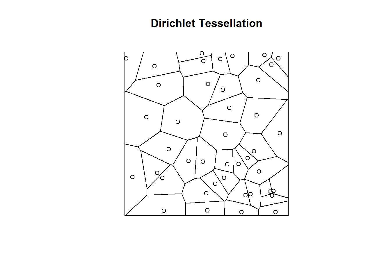

Figure 3.1: Dirichlet tesselation of \(\mathbb{R}^2\) using a set of randomly generated points.

Note that with either of these two approaches, the value of \(\lambda(s)\) needs to be evaluated at a sample of points distributed throughout the spatial domain, \(G\). Readers familiar with fitting species distribution models using MaxEnt or with estimating resource-selection functions using logistic regression hopefully see a connection here (i.e. the need for a representative sample from a well-defined spatial domain). Indeed, both MaxEnt and resource-selection functions have been shown to be equivalent to fitting an IPP model (Warton & Shepherd, 2010; Aarts et al., 2012; Fithian & Hastie, 2013; Renner & Warton, 2013; Renner et al., 2015), and it is useful to consider the background or available locations required by these methods as also approximating the integral in the IPP likelihood. This understanding, for example, suggests that the number of available points should be increased until the likelihood converges to a constant value (Warton & Shepherd, 2010; Renner et al., 2015).

3.5 Weighted Distributions: Connecting SHA Process Models to the IPP

Weighted distribution theory (Subhash R. Lele & Keim, 2006) provides a nice way to connect the SHA models discussed in Chapter 2 to the IPP model introduced here (Aarts et al., 2012). As in Chapter 2, let:

• \(f_u(x)\) = the frequency distribution of habitat covariates at locations where animals are observed.

• \(f_a(x)\) = the frequency distribution of habitat covariates at locations assumed to be available to our study animals.

We can think of the resource-selection function, \(w(x, \beta)\), as providing a set of weights that takes us from the distribution of available habitat in environmental space (\(E\)) to the distribution of used habitat (again, in \(E\)-space):

\[\begin{equation} f_u(x) = \frac{w(x,\beta)f_a(x)}{\int_{z \in E}w(z,\beta)f_a(z) dz} \tag{3.9} \end{equation}\]

The denominator of (3.9) ensures that the left hand side integrates to 1 and thus, \(f_u(x)\) is a proper probability distribution.

We can also write the model in \(G\)-space:

\[\begin{equation} f_u(s) = \frac{w(x(s),\beta)f_a(s)}{\int_{g \in G}w(x(g),\beta)f_a(g) dg} \tag{3.10} \end{equation}\]

In this case, \(f_u(s)\) tells us how likely we are to find an individual at location \(s\) in \(G\)-space, which depends on the environmental covariates associated with location \(s\), \(x(s)\). Typically, \(f_a(s)\) is assumed to be uniform (i.e. all areas within \(G\) are assumed to be equally available to the species). Then, if we let \(w(x(s), \beta) = \exp(x\beta)\), we end up with the conditional likelihood of the IPP model (eq. (3.4)) (Aarts et al., 2012).

Thinking in terms of weighted distributions will sometimes be advantageous. In particular:

1. it makes it immediately clear that we are modeling the spatial distribution of observed (or, for telemetry studies, ‘used’) locations, \(f_u(s)\), as a function of covariates (through \(w(x(s), \beta)\)), while assuming all habitat in \(G\) is equally available/accessible.

2. it highlights a potential issue with applying this modeling framework in the context of species distribution models in that not all habitat may be equally accessible. In later chapters, we will relax this assumption by modeling \(f_a(s)\) using non-uniform distributions, recognizing that nearby locations are more accessible than far away locations.

3.6 Simulation Example: Fitting the IPP model

To elucidate the above theoretical sections, we demonstrate how to simulate data from an IPP model. We then use the two approximations to the likelihood discussed above to see if we can recover the parameters used to simulate the data.

First, we create a landscape consisting of a risk and a resource. There are several ways to generate spatially correlated random variables. Here we simulate these environmental variables as independent unconditional Gaussian Random Fields using the functions in the fields package (Nychka, Furrer, Paige, & Sain, 2021). The resulting output will be formatted as a raster (i.e. a grid of values with an associated spatial extent and resolution or cell size). We can plot the roster using raster::spplot(env) (Fig. 3.2).

library(fields) # for generating a Gaussian random field
library(raster) # to work with rasters
library(dplyr) # for manipulating data

# Generate 2 covariates
grid<- list( x= 1:1000, y= 1:1000) 
  obj<- circulantEmbeddingSetup(grid, Covariance="Exponential", aRange=150)
risk<-  raster(circulantEmbedding(obj))
resource<-raster(circulantEmbedding(obj))
env <- stack(risk, resource) # environmental layers
names(env)<-c("risk", "resource")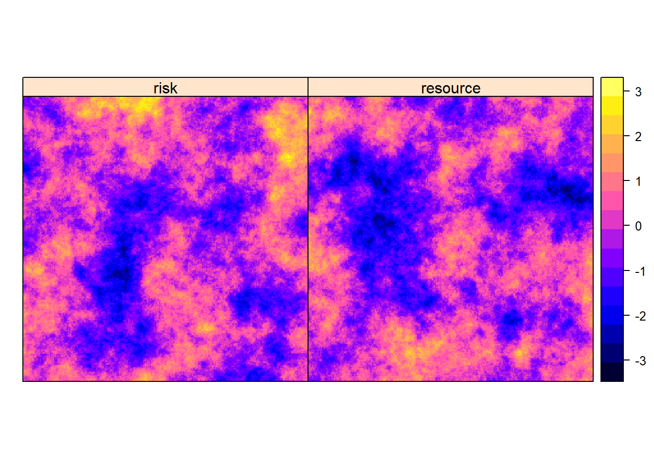

Figure 3.2: Geographical distribution of a risk (\(x_1\)) and resource (\(x_2\)) on a landscape.

We set the true intensity function to:

\[\log(\lambda(s)) = 6 - x_1(s) + 2x_2(s)\]

where \(x_1(s)\) and \(x_2(s)\) contain the values of the risk and resource, respectively, at each location, \(s\), within \(G\) (Fig. 3.2).

# Coefficients for the IPP model:
betas<-matrix(c(6,-1,2), nrow=3, ncol=1)
# Intensity function
lambdas<- exp(betas[1] + betas[2]*risk + betas[3]*resource)
# Point version
lambdas_m<-rasterToPoints(lambdas)

We then simulate random points within \(G\) using two steps:

1. We determine a random number of points, \(n_u\), to generate using the fact that \(n_u\) is a Poisson random variable with mean \(\mu = \int_G \lambda(s)ds\).

2. Conditional on having \(n_u\) points within \(G\), we determine their spatial locations by sampling from the original landscape (approximated here using a really fine grid) with cell probabilities proportional to \(\lambda(s)\) (eq. (3.4)).

Equivalently, we could have generated independent Poisson random variables for each cell in our fine grid (see Chapter 3.7.1 for more on the connection between gridded counts and the IPP model).

# Step 1: determine number of random points to generate
# mu = |G|mean(lambda(s)) over the spatial domain
# Area.G = area of the spatial domain
Area.G <- ((resource@extent@xmax-resource@extent@xmin)*(resource@extent@ymax-resource@extent@ymin))
mu <- cellStats(lambdas, stat='mean')*Area.G 
n_u <- rpois(1, lambda=mu) # number of points to generate
cat("mu = ", mu, "n_u = ", n_u)

## mu =  1421.823 n_u =  1473

# Step 2: determine their locations by sampling with
# probability proportional to lambda(s)
# x = design matrix holding the risk and resource values in the spatial domain
# n = number of grid cells in the spatial domain
# obs = index for each chosen observation
x <- cbind(rasterToPoints(env))
n <- nrow(x)
obs<-sample(1:n, size=n_u, prob=lambdas_m[,3], replace=TRUE)
# Step 3: create data frame with observed point-pattern
ppdat<-as.data.frame(x[obs,])

We can then look at the distribution of the locations in both G- and E-space (Figure 3.3).

gspace <- ggplot(data = ppdat, aes(x = x, y = y))+geom_point()+
     xlab("Easting")+ylab("Northing")+
     ggtitle("a. Geographical Space")
espace<- ggplot(data = ppdat, aes(x = risk, y = resource))+geom_point()+
     ggtitle("b. Environmental Space")
grid.arrange(gspace, espace, ncol=2)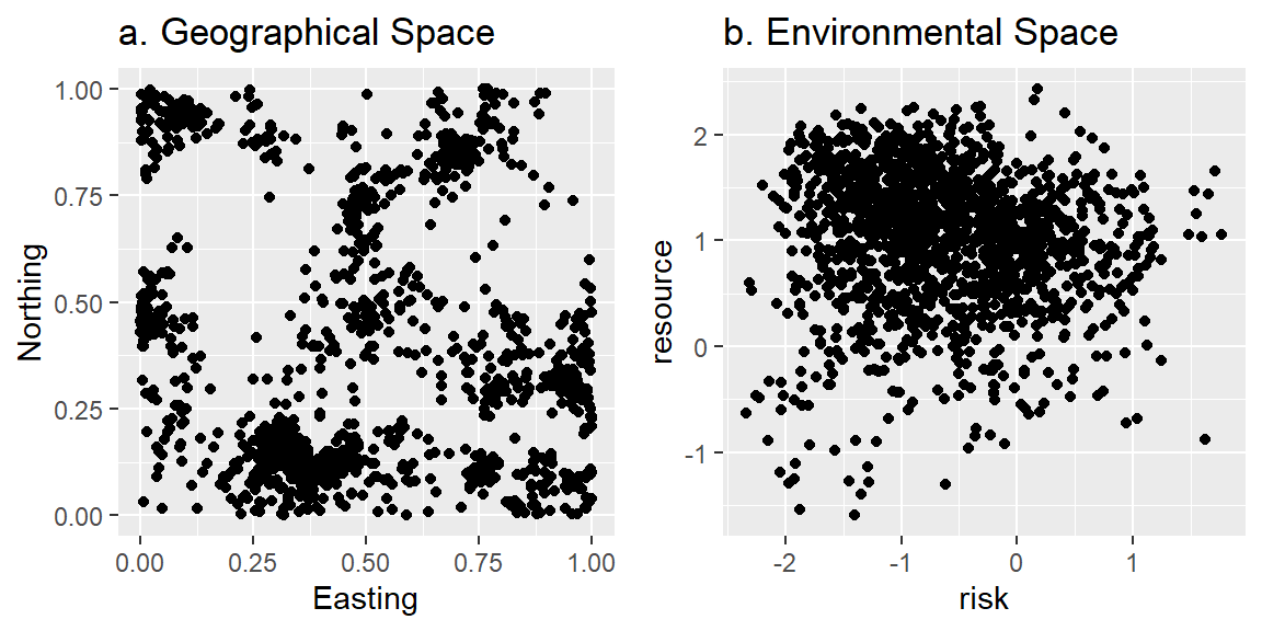

Figure 3.3: Plot of simulated locations in (a) geographical and (b) environmental space.

3.6.1 Maximum Likelihood Estimation (MLE) using Monte-Carlo Integration

To calculate the log-likelihood, we need to evaluate the intensity function at the observed points (eq. (3.6)). In addition, when estimating parameters using the approximation to the likelihood given by eq. (3.7), we will need to evaluate the intensity function at a set of random (available or background) points from within \(G\). We will use matrices and matrix multiplication to perform these calculations.⁹ We begin by creating a design matrix (xmat_u) for the observed points. Each row of the design matrix captures the values of the explanatory variables for one of the points. A column of 1’s is also included for the intercept (eq. (3.3)).

# Create design matrix containing covariates at observed locations
xmat_u <- cbind(1,ppdat[, c("risk", "resource")])
head(xmat_u, n=2) # Look at the first two observations

##   1      risk resource
## 1 1 -1.029812 1.413693
## 2 1 -1.593167 1.303835

We next generate a random sample of available points and create a design matrix for these points, xmat_a.

#' First, generate n_a random available points
n_a<-10000
randobs<-sample(1:n, size=n_a, replace=TRUE)
xmat_a <- cbind(1,x[randobs, c("risk", "resource")])
head(xmat_a, n=2)

##            risk  resource
## [1,] 1 1.913265  1.398941
## [2,] 1 0.453377 -1.696504

We then write a function to calculate the negative log-likelihood using Monte Carlo integration (eq. (3.7)).

logL_MC<-function(par, xmat_u, xmat_a, Area.G){
  betas<-par
# log(lambda) at observed locations for first term of logL 
# note %*% is used for matrix multiplication in R  
  loglam.u<-as.matrix(xmat_u) %*% betas
# lambda(s) at background locations for second term of LogL
  lambda.a<-exp(as.matrix(xmat_a) %*% betas)
# Now, sum terms and add a negative sign 
# to translate the problem from "maximization" to a "minimization" problem  
  -sum(loglam.u)+Area.G*mean(lambda.a) #negative log L
}

To find the values of \(\beta\) that minimize this function (equivalent to maximizing the likelihood), we will use the optim function in R, which offers a number of built-in optimization routines. optim requires a list of starting values for the numerical optimization routine (par = c(4, 0, 0)), the function to be minimized (logL_MC; note the first argument of this function needs to be the parameter vector that we are varying in order to find values that minimize our function), and an optimization method used to find the minimum (we choose to use BFGS but other options are also available). We can pass other arguments (e.g. xmat_u, xmat_a), which are needed in this case to calculate the negative log-likelihood at a given set of \(\beta\)’s.

#' Now estimate parameters:
mle_MC<-optim(par=c(4, 0, 0), fn=logL_MC, method="BFGS",
              xmat_u = xmat_u, xmat_a = xmat_a, Area.G = Area.G,
              hessian = TRUE)

The argument hessian=TRUE allows us to calculate asymptotic standard errors using standard theory for maximum likelihood estimators (Casella & Berger, 2002).¹⁰ The solve function in R will find the inverse of the Hessian, which provides an estimate of the variance-covariance matrix for our parameters. The square roots of the diagonal elements of this matrix give us our estimated standard errors.

varbeta_MC<-solve(mle_MC$hessian)
ests_MC<-data.frame(beta.hat=mle_MC$par, 
                    se.beta.hat=sqrt(diag(varbeta_MC)) )
#' Add the confidence limits to the data set using the mutate function
ests_MC <- ests_MC %>% mutate(lowerCI=beta.hat - 1.96*se.beta.hat,
                                upperCI=beta.hat + 1.96*se.beta.hat)
round(ests_MC, 2)

##   beta.hat se.beta.hat lowerCI upperCI
## 1     6.00        0.05    5.90    6.10
## 2    -1.01        0.04   -1.08   -0.94
## 3     2.06        0.04    1.98    2.14

We see that the parameters used to simulate the data, \((\beta_0, \beta_1, \beta_2) = (6, -1, 2)\) all fall within their respective 95% confidence intervals.

3.6.2 MLE using numerical integration

Alternatively, we could estimate parameters using the approximation to the likelihood given by eq. (3.8). To do so, we need to generate available locations on a regular grid and then determine appropriate quadrature weights. Quadrature weights reflect the area associated with the tile surrounding each available location and should sum to the total area of \(G\) which we have arbitrarily set to 1. We use the resolution of the sampled grid to determine the quadrature weights.

# Generate available data using a gridded background with
# n_a available points.
x_samp<-sampleRegular(env, size=n_a, asRaster=TRUE)
# Calculate quadrature weights:
# weights = delta x * delta y where delta x and deltay = size of grid cell 
weights <- xres(x_samp)*yres(x_samp)
cat("weights = ", weights, ";", "sum of weights = ", 
    sum(rep(weights, n_a)),  ";", 
    "area of omega =" , Area.G)

## weights =  1e-04 ; sum of weights =  1 ; area of omega = 1

We then create a design matrix for calculating the intensity function at the quadrature points.

#' Create design matrix containing covariates at background locations
xmat_a2<-cbind(1, rasterToPoints(x_samp)[, c("risk", "resource")])
head(xmat_a2, n=2) # look at the first two observations

##              risk  resource
## [1,] 1 -0.8045407 0.5393620
## [2,] 1 -1.1663175 0.6490776

We then write a function to calculate the negative log-likelihood for a given set of \(\beta\)’s, using the set of gridded available locations and their associated quadrature weights via eq. (3.8).

# Likelihood with numerical integration
logL_num<-function(par, xmat_u, xmat_a2,  weights){
  betas<-par
# log(lambda) at observed locations for first term of logL
  loglam.u<-as.matrix(xmat_u) %*% betas
# lambda(s) at background locations for second term of LogL
  lambda.a<-exp(as.matrix(xmat_a2) %*% betas)
# Now, calculate the negative log L  
  -sum(loglam.u)+sum(lambda.a*weights) 
}

And, again we use optim to minimize this function.

#Maximize likelihood
mle_num<-optim(par=c(4,0,0), fn=logL_num, method="BFGS",
               xmat_u = xmat_u, xmat_a2=xmat_a2,
               weights=weights, hessian=TRUE)
#' Estimates and SE's
varbeta_num<-solve(mle_num$hessian) # var/cov matrix of beta^
ests_num <- data.frame(beta.hat=mle_num$par, 
                       se.beta.hat=sqrt(diag(varbeta_num)))
#' Add the confidence limits to the data set using the mutate function
ests_num <- ests_num %>% mutate(lowerCI=beta.hat - 1.96*se.beta.hat,
                                upperCI=beta.hat + 1.96*se.beta.hat)
round(ests_num,2)

##   beta.hat se.beta.hat lowerCI upperCI
## 1     6.08        0.05    5.98    6.18
## 2    -0.95        0.04   -1.02   -0.88
## 3     1.98        0.04    1.91    2.06

We get nearly identical results as when using Monte Carlo integration, which is reassuring.

3.7 Fitting IPP models: Special Cases

3.7.1 Special Case I: Gridded Data

In many applications of SHA models, covariate data come from remote sensing data products that exist as a raster. In this case, we can estimate parameters of the IPP model by fitting a Poisson regression model to the count of individuals in each grid cell using the glm function in R (Aarts et al., 2012). A Poisson glm is appropriate because the IPP model implies that spatial locations of the individuals are independent and that the number of individuals in grid cell \(i\) is a Poisson random variable with mean, \(\mu_i = \int_{G_i} \lambda(s)ds\). When all predictors are grid-based, then \(\mu_i=\lambda_i |G_i|\), where \(\lambda_i\) is the value of \(\lambda(s)\) in grid cell \(i\) and \(|G_i|\) is the area of grid cell \(i\). This model could be specified using: glm(y ~ x + offset(log(area)), family = poisson()), where area measures the area of each grid cell. For readers that may not be familiar with an offset, this term is similar to including log(area) as a predictor, but forcing its coefficient to be 1. There are two reasons to include an offset: 1) it allows us to directly model densities (number of individuals per unit area); and 2) it provides a way to account for varying cell sizes in the case of irregular grids or meshes.

Let \(N_i\) and \(D_i\) represent the number and density of individuals in grid cell \(i\). We can formulate our model in terms of density:

\[\begin{gather} E[D_i] = \frac{E[N_i]}{G_i} = \lambda_i \\ \implies \log\left(\frac{E[N_i]}{|G_i|}\right)= \log(\lambda_i) \\ \implies \log(E[N_i]) - \log(|G_i|) = \log(\lambda_i) \\ \implies \log(E[N_i]) = \log(|G_i|) + \beta_0 + \beta_1x_1(s_i) + \ldots \beta_px_p(s_i) \tag{3.11} \end{gather}\]

If all cells are equally sized, then including an offset will only affect the intercept \(\beta_0\) but not the other regression parameters. In the case of unequal cell sizes, however, omitting the offset can lead to biased parameter estimates.

3.7.2 Special Case II: Presence-Absence Data

What if our usage data consists of binary (0 or 1) presence-absence data within the set of grid cells? Let’s assume the IPP model is again appropriate. Consider grid cell \(i\) that is of area \(|G_i|\), and let \(y_i\) = 1 if there is at least 1 observed individual in cell \(i\) and 0 otherwise. \(P(y_i = 1)\) is given by:

\[\begin{equation} P(y_i = 1) = 1- P(y_i = 0). \end{equation}\]

If the IPP model is appropriate, then the number of individuals in cell \(i\) is a Poisson random variable with mean \(\lambda_i|G_i| = \exp(\beta_0 + \beta_1x_1(s_i) + \ldots \beta_px_p(s_i))|G_i|\). Thus,

\[\begin{eqnarray} P(y_i = 0) & = & \frac{y_i^0\exp(-\lambda_i|G_i|)}{0!} \\ &=& \exp(-\lambda_i|G_i|) \end{eqnarray}\]

and, we have:

\[\begin{gather} P(y_i = 1) = p_i = 1- \exp(-\lambda_i|G_i|) \\ \implies p_i = 1- \exp(-\exp(\beta_0 + \beta_1x_1(s_i) + \ldots \beta_px_p(s_i))|G_i|) \end{gather}\]

Thus, it is natural to model binary presence-absence data using the so-called “complementary log-log link” (Baddeley et al., 2010):

\[\begin{equation} y_i \sim \mbox{Bernoulli}(p_i), \end{equation}\]

\[\begin{equation} \log(-\log(1-p_i)) = \beta_0 + \beta_1 x_1(s) + \ldots \beta_px_p(s) + log(|G_i|) \end{equation}\]

We can fit this model in R using:

glm(y~x1+x2+...xp + offset(log(area)), family=Binomial(link=cloglog))

Although it is more common to fit binary regression models with a logit link (i.e. \(\log(\frac{p_i}{1-p_i}) = x\beta\)), the complementary log-log link is appealing because of its connection with the IPP model. Further, it provides an opportunity to connect different types of usage data (presence-absence and point or count data) under a common process model (e.g. Fithian & Hastie, 2013; Koshkina et al., 2017; Scotson, Fredriksson, Ngoprasert, Wong, & Fieberg, 2017). Like the logit link, the complementary log-log link ensures \(p\) is constrained to lie between 0 and 1 as our predictor function goes from \(-\infty\) to \(\infty\) (Figure 3.4).

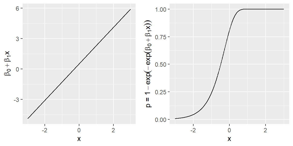
Figure 3.4: Plot of the predictor function and \(P(y=1)=p\) when using a complementary log-log link function with a single predictor x.

Note, although presence-absence data are frequently used to model species distributions, there is a potential loss of information when summarizing counts using binary observations. The loss of information by summarizing counts into binary observations becomes more severe when grid cells are large and species density is high. For example, consider the extreme scenario where all grid cells include at least one observed individual. In this case, there will be no spatial variation in species occurrence, and we will have lost the ability to estimate species-habitat associations. It is also important, though not always recognized, that models of the probability of occurrence are scale dependent unless formulated under a continuous point-process framework [i.e. with complementary log-log link and offset equal to the log cell size; Baddeley et al. (2010)]. This scale dependence, and potential loss of information, can easily be seen by binning our simulated count data using a series of coarsening cell sizes (see Figure 3.5). The expected counts and the probability of presence both depend on the size of the grid cell. In addition, the probability of presence approaches 1 as the size of the grid cells increases.

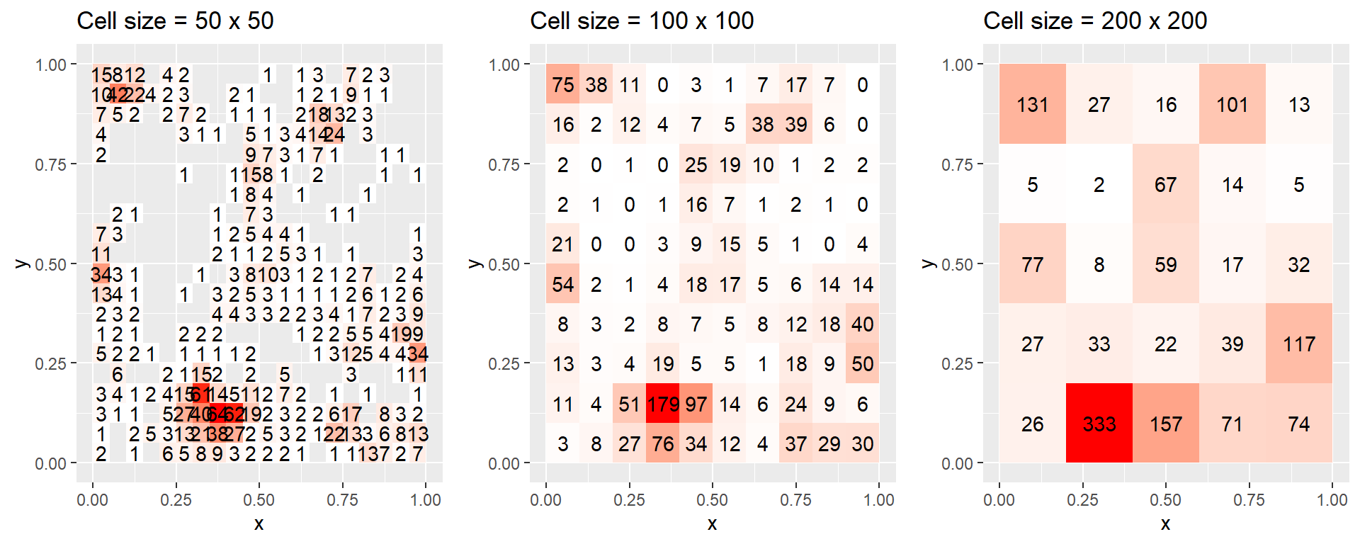
Figure 3.5: Gridded counts of the simulated locations shown in Figure 3.3a using grid cells of size a) 50 x 50, b) 100 x 100, and c) 200 x 200. Gray areas in panel (a) represent cells with 0 locations, which are too numerous to annotate. Note that the expected counts and the probability of presence both depend on the size of the grid cell, and the probability of presence approaches 1 as the size of the grid cells increases.

3.8 Imperfect Detection and Sampling Biases

The absolute density of observed individuals will often be driven by various observation-level processes (e.g. sampling effort, duration of data collection). In this case, our models effectively capture the density of sightings rather than the density of individuals on the landscape. As a result, the intercept in the IPP model is often difficult to interpret, and estimates of slope coefficients may be impacted by spatially varying observation biases. Given these issues, many applications of SHA models include covariates to adjust for observation biases and (rightly) abandon the idea of estimating absolute densities. In such cases, it can be convenient to work with the conditional likelihood of the IPP model [eq. (3.4); Aarts et al. (2012)] – i.e. the likelihood for the distribution of the locations as a function of covariates, conditional on having observed \(n_u\) locations. The conditional likelihood will also prove useful for extending our SHA model to address problems of unequal availability or accessibility of various habitats (see Section 3.5).

3.8.1 Conditional likelihood for IPP model

Here, we build on the simulation example from Section 3.6, demonstrating that we can recover the slope parameters by maximizing the conditional likelihood (eq. (3.4)), which we define below:

#' Conditional log-likelihood
logLCond<-function(par, xmat_u, xmat_a, MC=FALSE, weights=NULL){
  # MC = TRUE for Monte Carlo Integration
  # MC = FALSE for numerical integration
  betas<-par
  n<-nrow(xmat_u) # number of observed individuals
# log(lambda) at observed locations for first term of logL
# (use -1 to remove the term for the intercept)
  loglam.u<-as.matrix(xmat_u)[,-1] %*% betas
# lambda(s) at background locations for second term of LogL
  lambda.a<-exp(as.matrix(xmat_a)[,-1] %*% betas)
  if(MC==FALSE){
    -sum(loglam.u)+n*log(sum(lambda.a*weights)) #negative log L
  }else{
    -sum(loglam.u)+n*log(mean(lambda.a)) #negative log L
  }
}
# Using Monte Carlo Integration
mle_Cond_MC<-optim(par=c(0,0), fn=logLCond, method="BFGS",
                   xmat_u=xmat_u, xmat_a=xmat_a, MC=TRUE,
                   hessian=TRUE)
varbeta_Cond_MC<-solve(mle_Cond_MC$hessian)
ests_Cond_MC<-data.frame(beta.hat=mle_Cond_MC$par, 
                         se.beta.hat=sqrt(diag(varbeta_Cond_MC)) )

# Now using numerical integration
mle_Cond_NI<-optim(par=c(0,0), fn=logLCond, method="BFGS",
                   xmat_u = xmat_u, xmat_a=xmat_a2,
                   weights=weights, MC=FALSE, hessian=TRUE)
varbeta_Cond_NI<-solve(mle_Cond_MC$hessian)
ests_Cond_NI<-data.frame(beta.hat=mle_Cond_NI$par, 
                         se.beta.hat=sqrt(diag(varbeta_Cond_NI)) )

The results are nearly identical to those obtained from maximizing the full unconditional likelihood (Table 3.2).

Table 3.2: Estimates of Slope Parameters

Method	\(\hat{\beta_1}\)	SE	\(\hat{\beta_2}\)	SE
Full Monte Carlo	-1.01	0.04	2.06	0.04
Full Quadrature	-0.95	0.04	1.98	0.04
Conditional Monte Carlo	-1.01	0.04	2.06	0.04
Conditional Quadrature	-0.95	0.04	1.98	0.04

3.8.2 Thinned Point-Process Models

Our observations of habitat use will often be influenced by various sampling biases and uneven sampling effort [e.g. we may oversample areas near roads that are easily accessible by human observers; Sicacha-Parada, Steinsland, Cretois, & Borgelt (2020)]. These issues are particularly relevant to data collected haphazardly or opportunistically as part of museum collections or citizen science programs (Fithian et al., 2015). In such cases, it will often be fruitful to model the data as a thinned point-process model (Warton, Renner, & Ramp, 2013; Dorazio, 2014; Fithian et al., 2015; Sicacha-Parada et al., 2020). Specifically, we may think of the observed data as being generated by 2 processes: 1) the biological process model (as discussed in Chapter 2) written in terms of an Inhomogeneous Poisson Point-Process, and 2) an independent observation model that “thins” the data, specified using a separate function \(p(s)\) that describes the likelihood of observing an individual, conditional on that individual being present at location \(s\). Typically, \(p(s)\) will also be written as a log-linear function of spatial (and potentially non-spatial) covariates \((z_1, z_2, \ldots, z_m)\) and regression parameters \((\gamma_1, \gamma_2, \ldots, \gamma_m)\)¹¹:

\[log(p(s))= \gamma_0 + \gamma_1z_1(s) + \ldots \gamma_mz_m(s)\]

This leads to the following likelihood for the observed sightings:

\[\begin{equation} \log(L(\lambda, \beta \gamma |s_1, s_2, \ldots, s_n, n)) = \sum_{i=1}^{n}\log(\lambda(s_i)p(s_i)) - \int_G \lambda(s)p(s)ds \\ \tag{3.12} \end{equation}\]

If the covariates affecting \(\lambda(s)\) and \(p(s)\) are distinct, then we can think of the thinned point-process model as one where the intensity function includes both environmental drivers (\(x\)) and “observer bias variables” (\(z\)) (Warton et al., 2013). A benefit of the log-linear formulation of both \(\lambda(s)\) and \(p(s)\) is that it results in an additive model:

\[\begin{eqnarray} \log(\lambda(s)p(s)) & = & \log(\lambda(s))+\log(p(s)) \\ &=& (\beta_0 + \gamma_0) + \beta_1x_1(s) + \ldots \beta_px_p(s) + \gamma_1z_1(s) + \ldots \gamma_mz_m(s) \nonumber \tag{3.13} \end{eqnarray}\]

In this case, the intercepts of the two processes are not separately identifiable (i.e. we can only estimate their sum). Thus, we are unable to the model absolute intensity, \(\lambda(s)\), or absolute density of individuals. Similar issues arise if covariates influence both density and detectability, i.e. we will only be able to estimated the sum of these effects (but see Section 3.9 for possible solutions using data-integration techniques). If, on the other hand, the covariates that influence density and detectability are distinct, then we can obtain unbiased predictions for the distribution of locations, conditional on having observed a set of \(n_u\) locations, by setting the \(z\)’s to common values (Warton et al., 2013).

Quantitative ecologists have also developed a variety of methods to estimate absolute densities in situations where we cannot detect all individuals, but these methods will typically require specialized data collection methods (recall the Fisher quote from the start of this chapter) and additional modeling assumptions. We will demonstrate one of these approaches, distance sampling, in the next Section (3.8.3).

3.8.3 Simulation Example: Distance Sampling as a Thinned Point Process

To demonstrate fitting of a thinned point-process model, we will consider surveying our simulated individuals from Section 3.6 using a set of line transects. Specifically, we will place 40 equally-spaced transects throughout the survey region and assume:

1. all individuals that fall on the transect line are detected.
2. the probability of detecting individuals decreases with their distance from the transect line. A variety of models can be used to describe how detection drops with distance (Buckland et al., 2005). Here, we assume that detection probabilities follow a half-normal curve.

These assumptions result in a simple model for \(p(s)\), written in terms of a single covariate that depends on the perpendicular distance, \(z\), between each individual and the nearest transect line (Borchers & Marques, 2017)¹²:

\[\begin{equation} p(s) = \exp\left(\frac{-z(s)^2}{2\sigma^2}\right) \tag{3.14} \end{equation}\]

This formulation of the half normal model has one parameter, \(\sigma\), which determines how quickly detection probabilities decline with distance. It is also frequently used to model detection probabilities in spatial mark-recapture studies, with \(z(s)\) measuring the distance between an individual’s latent (i.e. unobserved) activity center and a set of traps (Royle, Chandler, Sun, & Fuller, 2013).

We can write our model for \(p(s)\) as a log-linear model:

\[\begin{equation} log(p(s)) = \gamma_0 + \gamma_1z_1(s) \tag{3.15} \end{equation}\]

with \(\gamma_0 = 0\) (to ensure \(p(s)=1\) for observations at 0 distance), \(z_1(s) = z(s)^2\), and \(\gamma_1 = 1/(2\sigma^2)\).

Here, we simulate data and show that we can again recover the parameters describing the intensity function. In the code below, we:

1. Place vertical transects along \(G\) using a systematic sampling design with a random starting location for the first transect.
2. Calculate perpendicular distances between each individual (\(s_1, s_2, \ldots, s_{511}\)) and the nearest transect to determine the probability of observing each individual.
3. Use a binomial random number generator to determine which of the \(n_u = 511\) individuals are observed.

# place 40 transects systematically with a random start
xminimum<-extent(resource)@xmin
xmaximum<-extent(resource)@xmax
transects.x<-seq(from=runif(1,xminimum,(xmaximum-xminimum)/40),to=xmaximum, length=40)
#transects.x<-seq(from=runif(1,0,/40),to=dim(resource)[1], length=40)
# determine distance between each observation and nearest
# transect
obs_x<-ppdat[, "x"] # x-coordinates of the n_u individuals
rownames(xmat_u)<-NULL # get rid of rownames and treat as data frame
xmat_u<-as.data.frame(xmat_u)
# Calculate perpendicular distance to nearest transect and square it
xmat_u$z<-sapply(1:n_u, FUN=function(x){min((obs_x[x]-transects.x)^2)})
# Determine detection probabilities using half-normal
sig <- 0.01 #
sig2<- sig*sig 
ps<-exp(-xmat_u$z/(2*sig2)) # p(s)
ppdat$detect<-rbinom(n_u, 1, ps)
#observed data
xmat_uobs<-xmat_u[ppdat$detect==1,]
# Available locations 
gridobs_x<-rasterToPoints(x_samp)[,1]
rownames(xmat_a)<-NULL
xmat_a_th<-as.data.frame(xmat_a)
# Add (distances to transects)^2 to the dataframe containing available data
xmat_a_th$z<-sapply(1:n_a, FUN=function(x){min((gridobs_x[x]-transects.x)^2)})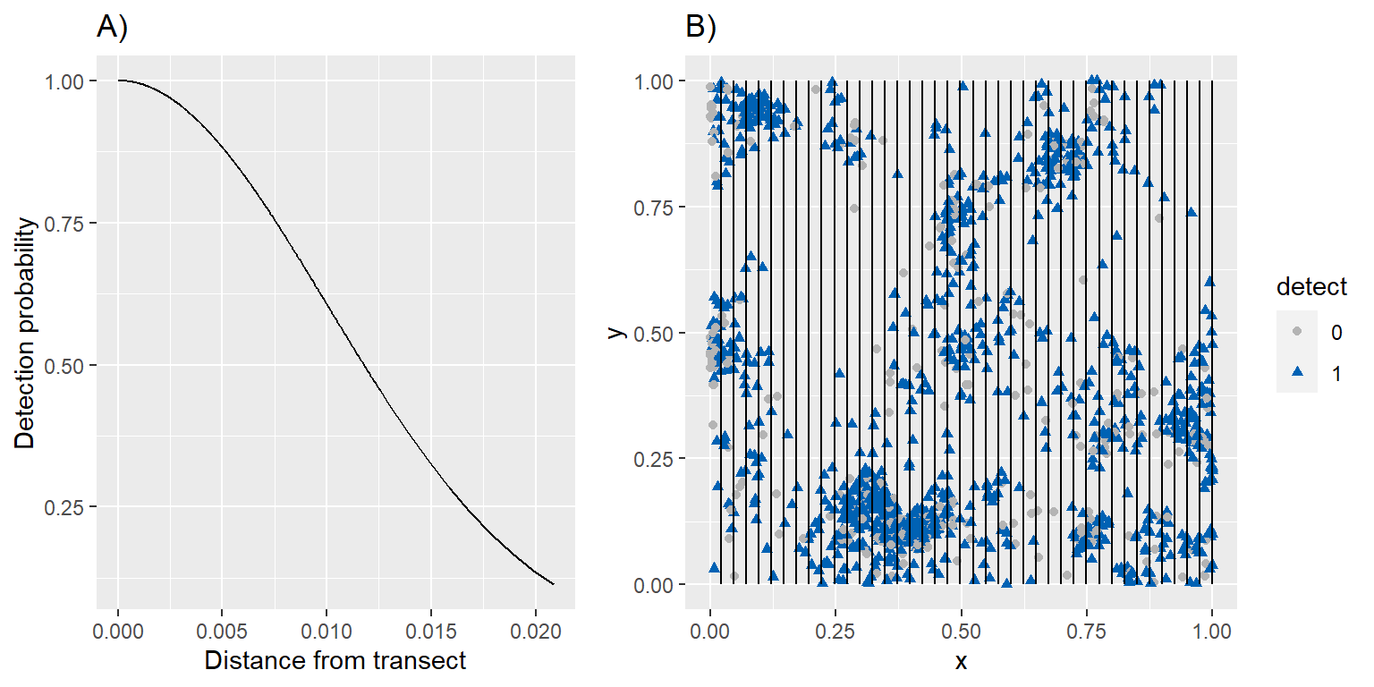

Figure 3.6: Distance sampling applied to the simulated data in Chapter 3. A) Detection probability as a function of distance from the transect line. B) Line transects (black lines) along with the underlying true and observed spatial point pattern.

Now, we write the likelihood of the thinned data and again use optim to estimate parameters of the process and observation model. To make sure that our estimate of \(\sigma\) is positive, we will parameterize the likelihood in terms of \(\theta = \log(\sigma)\), which implies \(\sigma = \exp(\theta)\).

LogL_thin<-function(pars, xmat_u, xmat_a, MC=FALSE, Area.G = 1, weights=NULL){
  # MC = TRUE for Monte Carlo Integration
  # MC = FALSE for numerical integration
  betas[1:3]<-pars[1:3] # parameters in lambda(s)
  sig <- exp(pars[4]) # par[4] = theta = log(sigma)
  betas[4]<- -1/(2*sig^2) 
  n<-nrow(xmat_u)
# log(lambda(s)*p(s)) at observed locations for first term of logL
  loglam.u<-as.matrix(xmat_u) %*% betas
# lambda(s)*p(s) at background locations for second term of LogL
  lambda.a<-exp(as.matrix(xmat_a) %*% betas) #second term
  if(MC==FALSE){ #quadrature
     -sum(loglam.u)+sum(lambda.a*weights) #negative log L
  }else{ # Monte Carlo integration
     -sum(loglam.u)+Area.G*mean(lambda.a) #negative log L
  }
}
mle_thin<-optim(par=c(4, 0,0,log(0.03)), fn=LogL_thin, method="BFGS",
              xmat_u = xmat_uobs, xmat_a=xmat_a_th, weights=weights, MC=FALSE,
              Area.G = Area.G, hessian=TRUE)
varbeta_thin<-solve(mle_thin$hessian)

Table 3.3: Estimates of IPP and Distance Sampling Parameters

Parameter	True value	Estiamte	SE
\(\beta_0\)	6.00	6.02	0.07
\(\beta_1\)	-1.00	-1.02	0.04
\(\beta_2\)	2.00	2.05	0.05
\(\sigma\)	0.01	0.01	0.06

We see (Table 3.3) that we are able to obtain accurate estimates of the parameters of the intensity function and the detection function. Note that it is the strong assumption of perfect detection on the transect line that allows us to estimate absolute density in this case. If this assumption fails, \(\gamma_0 \ne 0\) and we will underestimate density.

3.9 Looking Forward: Data Integration for Addressing Sampling Biases and Imperfect Detection

Of course, it is possible (and maybe quite likely) that \(\lambda(s)\) and \(p(s)\) will be influenced by one or more shared covariates (e.g. species that prefer forest cover may also be more difficult to detect when present in the forest compared to when they are in clearings). Unfortunately, in this case, we will not generally be able to separate out the effect of shared covariates on detection from their effect on species distribution patterns; we will only be able to estimate a single parameter for each shared covariate equal to \(\beta_i + \gamma_i\) (Dorazio, 2012; Fithian et al., 2015). There are some situations, however, where we can take advantage of multiple data sources and standardized survey protocols to estimate covariate effects on species distribution patterns in the presence of sampling biases. We mention a few possibilities here, but leave detailed discussions of these approaches to later chapters.

Quantitative ecologists have developed numerous methods for estimating detection probabilities in wildlife surveys (Lancia, Kendall, Pollock, & Nichols, 2005) \(-\) we saw one such approach in Section 3.8.3 (i.e. distance sampling). Other popular approaches typically require marked individuals or repeated sampling efforts either by multiple observers or the same observer at multiple points in time. Examples of methods that use marked individuals include spatial or non-spatial mark-recapture estimators (Royle, Chandler, Sollmann, et al., 2013; McCrea & Morgan, 2014) and sightability models (Steinhorst & Samuel, 1989; Fieberg, 2012; Fieberg, Alexander, Tse, & Clair, 2013). Methods that rely on repeated sampling include double-observer methods (e.g. Nichols et al., 2000), occupancy models (MacKenzie et al., 2017), and N-mixture models (Royle, 2004). These latter methods work by assuming population abundance (or presence-absence in the case of occupancy models) does not change between sampling occasions (referred to as an assumption of population closure). If this assumption holds, repeated sampling can provide the information necessary to model detection probabilities. In particular, if we see a species present at a site during one sampling occasion and not another, then we know that we failed to detect it during the latter occasion. N-mixture models work similarly, but rely on variability in counts over time to inform the model of detection probabilities. Yet, both approaches can break down when their assumptions, which are difficult to verify, do not hold (e.g. Welsh, Lindenmayer, & Donnelly, 2013; Barker, Schofield, Link, & Sauer, 2018; Link, Schofield, Barker, & Sauer, 2018).

Recently, there have been many efforts to integrate data from unstructured (“presence-only”) surveys with data from structured surveys that allow estimation of detection probabilities (see recent reviews by D. A. Miller et al., 2019; and Fletcher et al., 2019; Isaac et al., 2020). Data integration has the potential to increase spatial coverage, precision, and accuracy of estimators of species distributions (Pacifici, Reich, Miller, & Pease, 2019). Most often, data integration is done via a joint likelihood with shared parameters [e.g. treating the presence-only data as a thinned version of the same point-process model used to model data from structured surveys; Dorazio (2014); Fithian et al. (2015); Koshkina et al. (2017); Schank et al. (2017); Isaac et al. (2020)]. As an alternative to using joint likelihoods, Pacifici et al. (2017) suggested using “data fusion approaches” that share information by using one data set as a predictor when modeling another or by using spatial random effects that are shared across multiple data sets (see also Gelfand & Shirota, 2019; Gelfand, 2020). These latter approaches should be more robust to differences in underlying intensity functions since they make fewer assumptions about shared parameters, and they are also likely to be preferable in cases where one data source is clearly superior to others. Data may also be integrated across multiple species to infer spatial variability in detection probabilities, either using data from non-target species as a surrogate for survey effort (Manceur & Kühn, 2014) or through joint modeling under the assumption that observation processes are common to multiple species (e.g. Fithian et al., 2015; Giraud, Calenge, Coron, & Julliard, 2016; Coron, Calenge, Giraud, & Julliard, 2018). Other work in this area has included developing methods to deal with misaligned spatial data (Pacifici et al., 2019) and integrating data that are clustered in space (Renner, Louvrier, & Gimenez, 2019).

Simmonds, Jarvis, Henrys, Isaac, & O’Hara (2020) used simulations to evaluate the performance of different data integration frameworks when faced with small sample sizes, low detection probabilities, correlated covariates, and poor understanding of factors driving sampling biases. They found that data integration was not always effective at correcting for spatial bias, but that model performance improved when either covariates or flexible spatial terms were included to account for sampling biases. In another study, Fletcher et al. (2019) found that models fit to combined presence-only and standardized survey data were nearly identical to models fit to just the presence-only data due to their being much more presence-only than standardized data. Using cross-validation techniques, they found that weighted likelihoods led to improved predictions. Much work still needs to be done to evaluate the performance of various data integration methods under different data generating scenarios (Isaac et al., 2020; Simmonds et al., 2020).

3.10 Looking Forward: Relaxing the Independence Assumption

As discussed in Chapter 1, locations of individuals will often be clustered in space, and some of the clustering may be driven by demographic rather than environmental processes. A classic example is the clustering in space of forest communities driven by limited dispersal capabilities (Seidler & Plotkin, 2006). Autocorrelation is also an inherent property of telemetry data (as will be discussed in the next Section, 3.11). A key assumption of the Inhomogeneous Poisson Point-Process model is that any clustering of observations in space can be explained using spatial covariates. Or, in other words, locations of the individuals in the population are independent after conditioning on \(x(s)\). There are several ways that this assumption can be relaxed. In particular, there are formal point-process models that include various forms of dependence (attraction or repulsion of points), and several of these can be fit using functions in the spatstat library (Baddeley & Turner, 2005). For an example in the context of species distribution modeling, see Renner et al. (2015). Alternatively, we can allow for dependencies by adding a spatially correlated random effect, \(\eta(s)\), to the intensity function:

\[\begin{equation} \log(\lambda(s)) =\beta_0 + \beta_1x_1(s) + \ldots \beta_px_p(s) + \eta(s) \tag{3.16} \end{equation}\]

Usually, \(\eta(s)\) is modeled as a multivariate Gaussian process with \(E[\eta(s)]=0\) and \(Cov[\eta(s), \eta(s')]\) depending on the distance between \(s\) and \(s'\); we used a similar approach to simulate data in Section 3.6.¹³

Although adding spatially correlated random effects may at first appear to be a simple extension to the IPP model, these models can be more difficult to fit to real data, particularly in a frequentist framework (Renner et al., 2015). Thus, we will leave further consideration of these approaches until later chapters. We do, however, wish to make two more important points. First, there may be times when we are willing to estimate parameters (or summarize location data from each of several tagged individuals) using models that assume independence, but use alternative methods for calculating SE’s that are robust to the independence assumption [e.g. using a block or cluster-level bootstrap; Fieberg, Vitense, & Johnson (2020); Renner et al. (2015)]. Second, residual spatial correlation may differ across different data sets, and this may have important implications for integrated models that combine data under the assumption of a constant intensity function as discussed in Section 3.9 (see also Renner et al., 2019).

3.11 Telemetry data

3.11.1 Logistic Regression and Resource-Selection Functions

As briefly alluded to in the introduction of this chapter (Table 3.1), telemetry data differ from most survey data sets in that individuals are repeatedly followed over time. Despite this inherent difference, data from telemetry studies are often pooled and analyzed using methods similar to those described earlier in this chapter. In particular, logistic regression is often applied to data sets consisting of observed locations (with \(y_i = 1\)) and randomly generated background (referred to as available) locations (with \(y_i = 0\)). Logistic regression models are parameterized using a logit link \((i.e. \log(\frac{u}{1-u}))\) rather than complementary log-log link as described in Section 3.7.2:

\[\begin{equation} \log(P(Y_i =1 | x)/[1-P(Y_i=1|x)]) = \beta_0+\beta_1x_1(s)+ \beta_2x_2(s)+\ldots \beta_px_p(s) \tag{3.17} \end{equation}\]

Rather than use the inverse-logit transform \((\frac{e^\mu}{1+e^\mu})\) to estimate \(P(Y_i =1 | x)\), which largely reflects the number of available locations used to fit the model, most analyses of telemetry data focus on the exponential of the linear predictor without the intercept:

\[\begin{equation} \exp(\beta_1x_1(s)+ \beta_2x_2(s)+\ldots \beta_px_p(s)) \tag{3.18} \end{equation}\]

referred to as a resource-selection function (RSF) [Section 2.8; Boyce & McDonald (1999)].

Historically, RSFs were described as providing estimates of “relative probabilities of use.” We find this terminology problematic, however, since the probability of use requires first defining an appropriate spatial and temporal unit (e.g. use of a 100 km\(^2\) area over a 3-month time period); the probability of finding at least one telemetry location in a grid cell will increase as we increase the grid cell size or the length of a telemetry study (see discussion in Subhash R. Lele & Keim, 2006).

Ecologists debated for many years whether logistic regression was appropriate for analyzing use-availability data (e.g. Keating & Cherry, 2004; C. J. Johnson, Nielsen, Merrill, McDonald, & Boyce, 2006). Warton & Shepherd (2010) ended this debate by showing that the slope parameters of a logistic regression model will converge to those of an IPP model as the number of available points increases to infinity. The connection to the IPP model also clarified the role of available points in the model fitting process (they allow us to approximate the integral in the denominator of the IPP likelihood). With logistic regression, the used locations also contribute to this integral, but the contribution becomes negligible as the number of available locations increases. Fithian & Hastie (2013) later showed that convergence is only guaranteed if the model is correctly specified or if available points are assigned “infinite weights.” Therefore, when fitting logistic regression or other binary response models (e.g. boosted regression trees), one should assign a large weight (say 5000 or more) to each available location and a weight of 1 to all observed locations (larger values can be used to verify that results are robust to this choice). Alternatively, instead of increasing the contribution of the availability points to the integral, we can decrease the contribution of the used locations and switch to a Poisson likelihood function as discussed in Section 5, Supplement S1 of Renner et al. (2015). The potential advantage of this approach is that it then becomes possible to estimate the intercept, and thus, the absolute density of observations.

To demonstrate that infinitely-weighted logistic regression and down-weighted Poisson regression can be used to estimate parameters in an IPP model, we apply these approaches to our simulated data from Section 3.6. We begin with infinitely-weighted logistic regression:

# Create a data frame with used and available locations
rsfdat<-rbind(xmat_u[,c("risk", "resource")], xmat_a[, c("risk", "resource")])
# Create y (1 if used, 0 otherwise)
rsfdat$y<-c(rep(1, nrow(xmat_u)),rep(0, nrow(xmat_a)))
# Assign large weights to available locations
rsfdat$w<-ifelse(rsfdat$y==0,5000,1)
# Fit weighted logistic model and look at summary
rsf<-glm(y~risk+resource, data=rsfdat, weight=w, family=binomial())

We see that we get identical estimates of the coefficients and their SEs as obtained when fitting the IPP model using the conditional likelihood (compare Tables 3.2, 3.4).

To implement the down-weighted Poisson approach, we create small weights (\(w= 1^{-6}\)) for the observed locations and weights equal to the area sampled divided by the number of random points (\(w=\frac{|G|}{n_a}\)) for the available locations. We then model \(Y_i = 0\) for the available locations or \(Y_i = 1/w\) for the observed locations.

# A = area sampled
A=1 
# Create weights
rsfdat$w2<-ifelse(rsfdat$y==0, A/sum(rsfdat$y==0), 1.e-6)
# Fit down-weighted Poisson regression model
rsfDWP<-glm(y/w2~risk+resource, data=rsfdat, weight=w2, family=poisson())

Table 3.4: Regression coefficients in infinitely-weighted logistic and down-weighted Poisson regression models fit to simulated data.

	Infinitely-weighted Logistic		Down-weighted Poisson
	Estimate	Std. Error	Estimate	Std. Error
(Intercept)	NA	NA	6.02	0.05
risk	-1.01	0.04	-0.99	0.04
resource	2.06	0.04	2.03	0.04

We see that we again recover the parameter values used to simulate the data, including the intercept (Table 3.4).

3.11.2 Connection to Utilization Distributions and Animal Home Ranges

In the context of home-range modeling, the distribution of habitat use in geographic space, \(f_u(s)\), is often refereed to as a utilization distribution (Jennrich & Turner, 1969; Van Winkle, 1975). We can estimate this distribution directly using various non-parametric methods, including 2-dimensional kernel density estimators (Figure 3.7).

# Create data set with locations (x,y)
dataHR = as.data.frame(x[obs,c("x","y")])
# Calculate and plot 2-D density estimate f_u(s) using kde
H <- ks::Hpi(dataHR)

Figure 3.7: Kernel density estimate of \(f_u(s)\) (z-axis) for the simulated point pattern data in Figure 3.3; \(f_u(s)\) depicts the distribution of habitat use in geographic space, also known as the utilization distribution.

In Section 2.9, we demonstrated that we can also estimate \(f_u(s)\) using a fitted RSF. What we omitted at the time, however, was that we first need to determine an appropriate spatial domain of availability, \(G\), in geographic space. It is common to estimate \(G\) using a minimum convex polygon or the 95% isopleth of a kernel density estimator (KDE) applied to an individual’s locations in geographic space (Figure 3.8); these same methods are frequently used to determine an outer contour when estimating the size of an individual’s home range (see e.g. Worton, 1989; Kie et al., 2010; Fieberg & Börger, 2012; Horne et al., 2020).

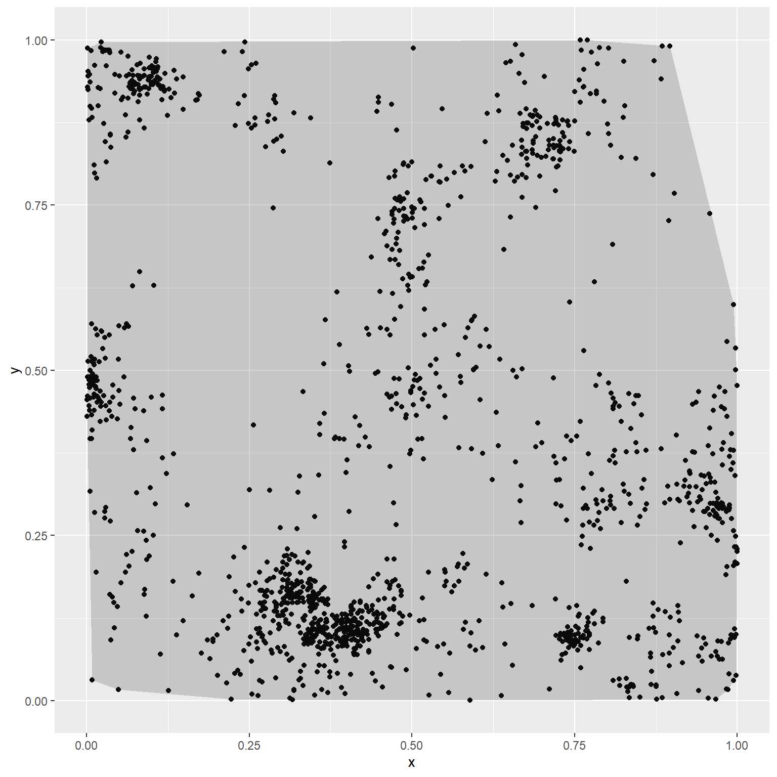
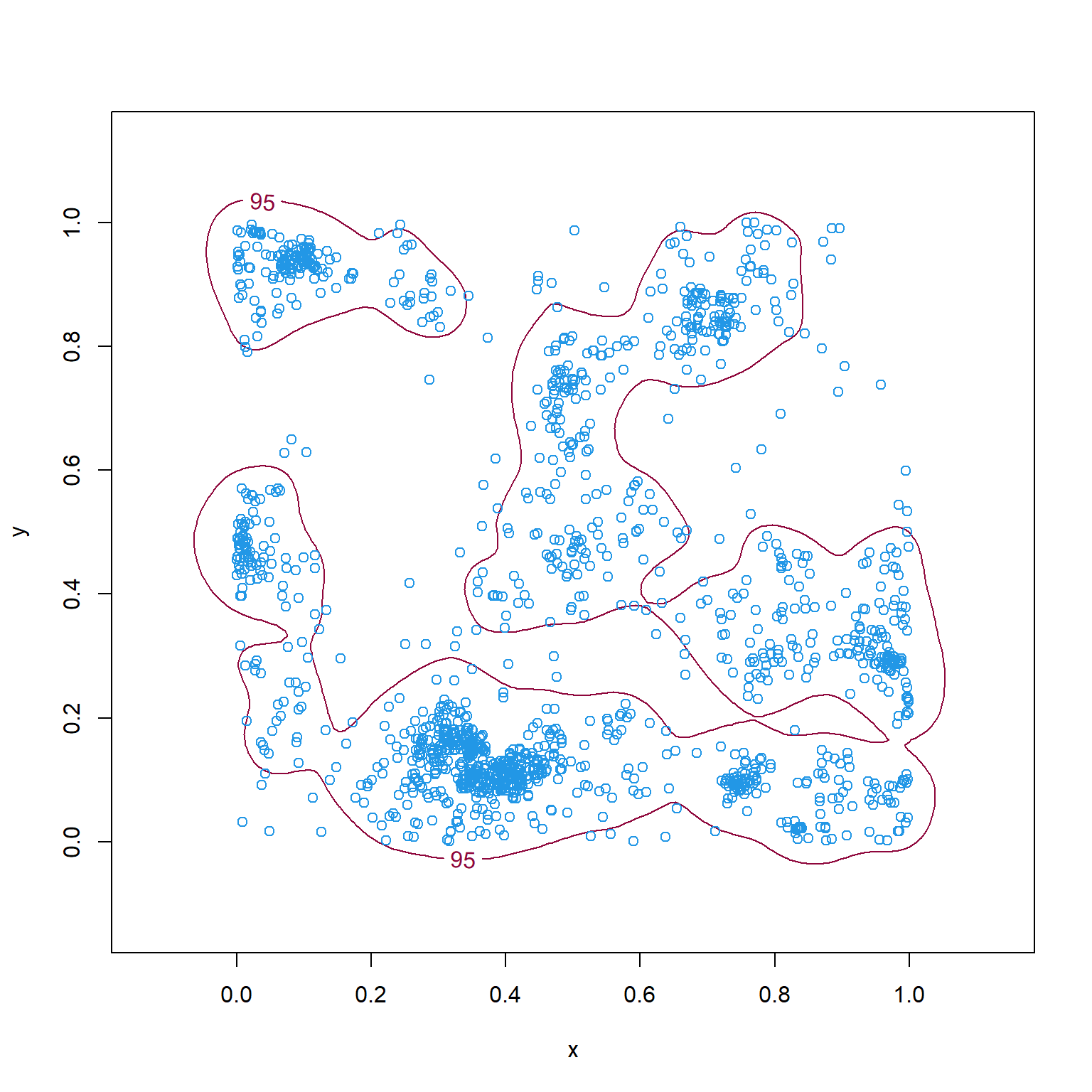
Figure 3.8: Minimum convex polygon (left) and 95th percentile isopleth of a kernel density estimate of \(f_u(s)\) (right) for the simulated point pattern data in Chapter 3.

Once we have determined an appropriate domain of habitat availability, \(G\), we can fit an IPP model using the methods described in this chapter. We can then estimate \(f_u(s)\) using eq. (3.10) as demonstrated in Section 2.9.

Although the RSF approach allows us to model \(f_u(s)\) as a function of spatial predictors, it is somewhat circular since we have to first estimate \(G\) (often with an initial estimate of \(f_u(s)\) obtained from a KDE) before estimating \(\beta\), \(w(x(s), \beta)\), and then \(f_u(s)\) again via equation (3.10). Others have suggested estimating \(f_u(s)\) using a KDE, which then may be regressed against spatial predictors to infer the importance of environmental characteristics on habitat use (Marzluff, Millspaugh, Hurvitz, & Handcock, 2004; Millspaugh et al., 2006). This approach, when used with a log-transformation, can again be shown to approximate an IPP model (Hooten, Hanks, Johnson, & Alldredge, 2013). Alternatively, Horne, Garton, & Rachlow (2008) suggested we should simultaneously estimate parameters in \(f_a(s)\) and \(w(x(s), \beta)\) by directly maximizing the weighted distribution likelihood formed using eq. (3.10). Horne et al. (2008) referred to this approach as fitting a synoptic model since it models space use by incorporating both home-range and resource-selection processes. If we assume \(f_a(s)\) is described by bi-variate normal distribution, \(\Phi(s, \mu, \sigma^2)\), then we can simultaneously estimate the mean (\(\mu\)) and variance parameters (\(\sigma^2\)) in \(f_a(s)\) and the regression parameters in \(w(x(s), \beta)\) by maximizing the likelihood given by eq. (3.19):

\[\begin{equation} L(\mu, \sigma, \beta|s_1, \ldots, s_n) = \prod_{i=1}^{n}\frac{w(x(s_i), \beta)\Phi(s_i, \mu, \sigma^2)}{\int _{g \in G} w(x(g), \beta)\Phi(g, \mu, \sigma^2)dg} \tag{3.19} \end{equation}\]

As with IPP models, the integral in the likelihood must be approximated using Monte Carlo or numerical integration techniques. The same approach has been used to motivate a joint likelihood model for integrating telemetry data and spatial mark-recapture data (Royle, Chandler, Sun, et al., 2013).

In the home-range literature, an important distinction has been made between the distribution of locations an animal uses during a specific observation window, referred to as an occurrence distribution, and the asymptotic (or equilibrium) distribution that results from assuming animals move consistently in a range-restricted manner, referred to as the range distribution (Fleming et al., 2015, 2016; Horne et al., 2020). These two distributions represent different statistical estimation targets, which has important implications when choosing a home-range estimator and when considering the effect of autocorrelation on home-range estimators (Fleming et al., 2014; Noonan et al., 2019). Autocorrelation is an asset when estimating the occurrence distribution using time-series kriging, a method that uses autocorrelation to better predict “nearby” locations in time (Fleming et al., 2016). On the other hand, autocorrelation may impact effective sample sizes and thus optimal levels of smoothing when using kernel density estimators to estimate the range distribution (Fleming et al., 2015).

This distinction between describing, retrospectively, the distribution of habitat used by an animal and, prospectively, the distribution of habitat that an animal will likely use in the future has received less attention in the SHA literature. Our view is that RSFs capture historic habitat use (analogous to an occurrence distribution), which when combined across various sampling instances, can provide insights that may allow us to predict future habitat use in novel environments. In later chapters we will encounter movement-based habitat selection models that can be used to generate predictive distributions of animal space-use in novel environments. In both cases, we will need to consider the role autocorrelation plays in determining appropriate estimators, including estimators of parameter uncertainty.

3.11.3 Looking Forward: Non-Independence of Telemetry Locations

As alluded to in the previous section, it is important to consider whether the assumption that observed locations are independent is reasonable when modeling home ranges or habitat selection from telemetry data. Strictly speaking, this assumption will almost never be met, particularly with modern-day telemetry studies that allow several locations to be collected on the same day. In particular, observations close in time are likely to be close in space (Aarts et al., 2008; Fleming et al., 2014). Elsewhere Fieberg (2007) argued that a representative sample of locations may be sufficient for consistent (asymptotically unbiased) estimation of utilization distributions that describe habitat use during a fixed observation window (e.g. a breeding season or annual cycle), analogous to estimating the occurrence distribution. Similarly, if telemetry observations are collected regularly (or randomly) in time, then the locations may be argued to provide a representative sample of habitat use from a specific observation window. In these cases, it may be helpful to view our estimates of RSF parameters, \(\hat{\beta}\), as useful summaries of habitat use for tagged individuals during these fixed time periods. The question then becomes, how should we use these summaries to make inferences about a population or species? The assumption of independence of our locations is clearly problematic, and ignoring statistical dependence will bias our estimates of uncertainty. What should we do about this? We have a few options:

1. Calculate a time to independence between observations and either down-weight the contribution of each observation or subsample from the autocorrelated observations to obtain an independent sample (Swihart & Slade, 1985). Yet, subsampling involves the removal of valuable data, and it may not always be possible to achieve independence through subsampling (Noonan et al., 2020).
2. If we are interested in population-level summaries of habitat use, then we may choose to ignore within-individual autocorrelation when estimating individual-specific coefficients, but use a robust form of SE that treats individuals as independent when describing uncertainty in population-level parameters (e.g. Craiu, Duchesne, & Fortin, 2008; Fieberg, Matthiopoulos, Hebblewhite, Boyce, & Frair, 2010).
3. Alternatively, we may be able to address issues related to autocorrelation by choosing a framework that allows us to model habitat selection and animal movement together (Hanks, Hooten, Alldredge, et al., 2015; Signer, Fieberg, & Avgar, 2017, 2019). These approaches can then be combined with hierarchical modeling frameworks that allow for individual-specific coefficients (Muff, Signer, & Fieberg, 2020). We will revisit these ideas in later chapters of the book.

An advantage of the last approach is that it provides a mechanistic link between spatial covariates and animal movements, which can be used to explore space-use patterns in novel environments (Signer et al., 2017; Michelot, Blackwell, & Matthiopoulos, 2019).

3.12 Camera Traps

Camera traps have become a popular and relatively inexpensive tool for monitoring the use of habitats by multiple species (O’Connell, Nichols, & Karanth, 2010; Wearn & Glover-Kapfer, 2019). Data from camera traps have been analyzed in many different ways (for an overview, see Sollmann, 2018), but it is not uncommon to fit models to counts of observations per unit time or to binary (detect/non-detect) summaries created for pre-specified time periods (e.g. days). Both approaches can be formulated in terms of an underlying spatial point-process or spatial-temporal point-process model. This feature has facilitated joint modeling of camera trap and other survey data (e.g. Scotson et al., 2017; Bowler et al., 2019). If individuals can be uniquely identified, then it is possible to fit spatial-mark-recapture models to camera trap data as thinned point processes (Borchers & Marques, 2017); it is also possible to integrate camera trap and telemetry data using a joint likelihood approach (Royle, Chandler, Sun, et al., 2013; Proffitt et al., 2015; Sollmann, Gardner, Belant, Wilton, & Beringer, 2016; Linden, Sirén, & Pekins, 2018). Given the ubiquity of camera trap data, we expect to see further development of approaches to integrating camera trap data with other data types in the future.

One important consideration when fitting models to camera trap data is that cameras sample very small areas defined by the camera’s field of view, and therefore, effectively sample points in space. Thus, although camera trap data are often analyzed using occupancy models, there is no clear connection to a “site” with well-defined spatial extent (Sollmann, 2018). Further, interpretation of estimates of occupancy is challenging since this metric will be influenced by both density of individuals and their average home-range size (Efford & Dawson, 2012; but see Steenweg, Hebblewhite, Whittington, Lukacs, & McKelvey, 2018 for an alternative point of view). Another important feature to consider when analyzing camera trap data (or other mark-recapture data) is whether or not lures or attractants have been used to increase detection rates (see e.g. Garrote et al., 2012; Braczkowski et al., 2016; Iannarilli, Erb, Arnold, & Fieberg, 2017; Maxwell, 2018; Mills, Fattebert, Hunter, & Slotow, 2019). These effects should also be considered when modeling habitat use-data as they may induce clustering rather than a thinning of observed data.

3.13 Software for fitting IPP models

In this chapter, we have demonstrated how the IPP model can be fit to simulated data using the full likelihood, conditional (weighted distribution theory) likelihood, and using infinitely-weighted logistic regression or down-weighted Poisson regression. Here, we briefly mention open-source software available for fitting the IPP model to spatial usage data. Advantages and disadvantages of different options for fitting IPP models are discussed in more detail in Renner et al. (2015), and we encourage interested readers to follow up by reading their paper (along with its associated supplementary material).

• the spatstat package in R uses numerical integration to fit a wide range of point-process models, including models that allow for clustering or competition in space (Baddeley & Turner, 2005). An advantage of using the spatstat library is that it also has built-in functions for evaluating model assumptions (e.g. point independence) and fit of the model (e.g. using residual plots). These functionalities will be illustrated in a later chapter.

• the ppmlasso package in R provides methods for fitting a range of spatial point-process models while also using regularization techniques to constrain model complexity and avoid overfitting.

• MaxEnt is a popular software program for fitting species distribution models using a maximum entropy approach (Phillips & Dudik, 2008; Merow et al., 2013). This approach is equivalent to fitting a Poisson process model but using highly flexible predictors to allow for complex species-habitat associations (non-linear responses and interactions). As with ppmlasso, a penalization term is used to constrain model complexity. MaxEnt also includes nice graphical features that allow one to explore areas in geographical space that require extrapolating outside the range of the data used to fit the model, and to evaluate which predictors are driving the predictions at any location in space. It is possible to fit models using MaxEnt using the dismo package in R (Hijmans, Phillips, Leathwick, & Elith, 2017).

• INLA is a general purpose Bayesian software platform that approximates posterior marginal distributions using integrated nested Laplace approximations rather than using Markov chain Monte Carlo (MCMC) sampling. It has become a popular method for fitting spatial models in a Bayesian framework (Illian, Sørbye, & Rue, 2012; Lindgren et al., 2015). The INLA (Lindgren & Rue, 2015) and inlabru (Yuan et al., 2017) R packages makes it is possible to fit models using INLA via an R interface (for more information about INLA, see: http://www.r-inla.org/ and for inlabru see https://inlabru-org.github.io/inlabru/index.html).

• The glmmTMB package in R (Brooks et al., 2017) can be used to fit linear and generalized linear mixed models using maximum likelihood via Template Model Builder (TMB) (Kristensen, Nielsen, Berg, Skaug, & Bell, 2015). TMB uses automatic differentiation to calculate likelihood gradients, which makes it easier to fit complex models. glmmTMB can fit IPP models to use-availability data via infinitely-weighted logistic regression or down-weighted Poisson Regression (Renner et al., 2015). Similar to INLA, glmmTMB can include spatial random effects using a Laplace approximation. The appeal is that it is relatively stable and fast for larger data sets.

3.14 Concluding remarks

In this chapter, we introduced the Inhomogeneous Poisson Point-Process model as a general framework for modeling species distributions. The IPP model allows us to work with and integrate several different data types (point locations, presence-absence data, gridded counts), while also accounting for observation and sampling biases via a thinning process. Thus, it provides a solid statistical foundation that allows us to link organisms to their habitat. In fact, it can be shown that most methods for modeling species distributions, including MaxEnt and resource-selection functions, are equivalent to fitting an IPP model. Nonetheless, it is important to recognize limitations and inherent challenges with interpreting the output of these models biologically. As discussed in Chapter 1, there are many reasons why the density of a species may not accurately reflect habitat suitability or fitness. Furthermore, there is a tendency among practitioners to approach model building with little thought \(-\) i.e. pass whatever remotely-sensed variables are available to MaxEnt, and let it construct an extremely flexible model that allows the “data to speak”. There are many issues with this approach. In addition to ignoring sampling biases (Yackulic et al., 2013), machine learning approaches are likely to lead to overfit models that do not transfer well to other locations (Fourcade et al., 2018). As we argued in Chapter 2, it is important to carefully consider biological mechanisms when building process models; classifying predictors as resources, risks, or conditions allows us to anticipate the functional relationship between predictors and fitness and is an important first step to building more realistic process models. This simple step may take us quite far when density is proportional to fitness (i.e. when our null model in Chapter 1 is appropriate). Unfortunately, the null model will often not be appropriate, and thus, future chapters will be devoted to relaxing its assumptions.

References

Aarts, G., Fieberg, J., & Matthiopoulos, J. (2012). Comparative interpretation of count, presence-absence and point methods for species distribution models. Methods in Ecology and Evolution, 3(1), 177–187. doi:10.1111/j.2041-210X.2011.00141.x

Aarts, G., MacKenzie, M., McConnell, B., Fedak, M., & Matthiopoulos, J. (2008). Estimating space-use and habitat preference from wildlife telemetry data. Ecography, 31(1), 140–160. doi:10.1111/j.2007.0906-7590.05236.x

Baddeley, A., Berman, M., Fisher, N., Hardegen, A., Milne, R., Schuhmacher, D., et al.others. (2010). Spatial logistic regression and change-of-support in Poisson point processes. Electronic Journal of Statistics, 4, 1151–1201. doi:doi:10.1214/10-EJS581

Baddeley, A., & Turner, R. (2005). spatstat: An R package for analyzing spatial point patterns. Journal of Statistical Software, 12(6), 1–42. doi:10.18637/jss.v012.i06

Barker, R. J., Schofield, M. R., Link, W. A., & Sauer, J. R. (2018). On the reliability of n-mixture models for count data. Biometrics, 74(1), 369–377. doi:10.1111/biom.12734

Borchers, D. L., & Marques, T. A. (2017). From distance sampling to spatial capture–recapture. AStA Advances in Statistical Analysis, 101(4), 475–494.

Bowler, D. E., Nilsen, E. B., Bischof, R., O’Hara, R. B., Yu, T. T., Oo, T., … Linnell, J. D. (2019). Integrating data from different survey types for population monitoring of an endangered species: The case of the eld’s deer. Scientific Reports, 9(1), 7766.

Boyce, M. S., & McDonald, L. L. (1999). Relating populations to habitats using resource selection functions. Trends in Ecology & Evolution, 14(7), 268–272.

Braczkowski, A. R., Balme, G. A., Dickman, A., Fattebert, J., Johnson, P., Dickerson, T., … Hunter, L. (2016). Scent lure effect on camera-trap based leopard density estimates. PLoS One, 11(4), e0151033.

Brooks, M. E., Kristensen, K., van Benthem, K. J., Magnusson, A., Berg, C. W., Nielsen, A., … Bolker, B. M. (2017). glmmTMB balances speed and flexibility among packages for zero-inflated generalized linear mixed modeling. The R Journal, 9(2), 378–400.

Buckland, S. T., Anderson, D. R., Burnham, K. P., & Laake, J. L. (2005). Distance sampling. In P. Armitage & T. Colton (Eds.), Encyclopedia of biostatistics (Vol. 2). Chichester, UK: Wiley Online Library. doi:10.1002/0470011815.b2a16019

Casella, G., & Berger, R. L. (2002). Statistical inference (Vol. 2). Duxbury Pacific Grove, CA.

Coron, C., Calenge, C., Giraud, C., & Julliard, R. (2018). Bayesian estimation of species relative abundances and habitat preferences using opportunistic data. Environmental and Ecological Statistics, 25(1), 71–93.

Craiu, R. V., Duchesne, T., & Fortin, D. (2008). Inference methods for the conditional logistic regression model with longitudinal data. Biometrical Journal: Journal of Mathematical Methods in Biosciences, 50(1), 97–109.

Dorazio, R. M. (2012). Predicting the geographic distribution of a species from presence-only data subject to detection errors. Biometrics, 68(4), 1303–1312. doi:10.1111/j.1541-0420.2012.01779.x

Dorazio, R. M. (2014). Accounting for imperfect detection and survey bias in statistical analysis of presence-only data. Global Ecology and Biogeography, 23(12), 1472–1484. doi:10.1111/geb.12216

Efford, M. G., & Dawson, D. K. (2012). Occupancy in continuous habitat. Ecosphere, 3(4), 1–15.

Fieberg, J. (2007). Kernel density estimators of home range: Smoothing and the autocorrelation red herring. Ecology, 88(4), 1059–1066.

Fieberg, J. (2012). Estimating population abundance using sightability models: R SightabilityModel package. Journal of Statistical Software, 51(9), 1–20.

Fieberg, J., Alexander, M., Tse, S., & Clair, K. S. (2013). Abundance estimation with sightability data: A Bayesian data augmentation approach. Methods in Ecology and Evolution, 4(9), 854–864.

Fieberg, J., & Börger, L. (2012). Could you please phrase ‘home range’ as a question? Journal of Mammalogy, 93(4), 890–902.

Fieberg, J., Matthiopoulos, J., Hebblewhite, M., Boyce, M. S., & Frair, J. L. (2010). Correlation and studies of habitat selection: Problem, red herring or opportunity? Philosophical Transactions of the Royal Society of London B: Biological Sciences, 365(1550), 2233–2244. Retrieved from http://www.pubmedcentral.nih.gov/articlerender.fcgi?artid=2894958\&tool=pmcentrez\&rendertype=abstract

Fieberg, J., Vitense, K., & Johnson, D. H. (2020). Resampling-based methods for biologists. PeerJ, 8, e9089. doi:10.7717/peerj.9089

Fithian, W., Elith, J., Hastie, T., & Keith, D. A. (2015). Bias correction in species distribution models: Pooling survey and collection data for multiple species. Methods in Ecology and Evolution, 6(4), 424–438. doi:10.1111/2041-210X.12242

Fithian, W., & Hastie, T. (2013). Finite-sample equivalence in statistical models for presence-only data. The Annals of Applied Statistics, 7(4), 1917. doi:10.1214/13-AOAS667

Fleming, C. H., Calabrese, J. M., Mueller, T., Olson, K. A., Leimgruber, P., & Fagan, W. F. (2014). From fine-scale foraging to home ranges: A semivariance approach to identifying movement modes across spatiotemporal scales. The American Naturalist, 183(5), E154–E167.

Fleming, C. H., Fagan, W. F., Mueller, T., Olson, K. A., Leimgruber, P., & Calabrese, J. M. (2015). Rigorous home range estimation with movement data: A new autocorrelated kernel density estimator. Ecology, 96(5), 1182–1188.

Fleming, C. H., Fagan, W. F., Mueller, T., Olson, K. A., Leimgruber, P., & Calabrese, J. M. (2016). Estimating where and how animals travel: An optimal framework for path reconstruction from autocorrelated tracking data. Ecology, 97(3), 576–582.

Fletcher, R. J., Hefley, T. J., Robertson, E. P., Zuckerberg, B., McCleery, R. A., & Dorazio, R. M. (2019). A practical guide for combining data to model species distributions. Ecology, 100(6), e02710. doi:10.1002/ecy.2710

Fourcade, Y., Besnard, A. G., & Secondi, J. (2018). Paintings predict the distribution of species, or the challenge of selecting environmental predictors and evaluation statistics. Global Ecology and Biogeography, 27(2), 245–256. doi:10.1111/geb.12684

Garrote, G., Gil-Sánchez, J. M., McCain, E. B., Lillo, S. de, Tellería, J. L., & Simón, M. Á. (2012). The effect of attractant lures in camera trapping: A case study of population estimates for the iberian lynx (lynx pardinus). European Journal of Wildlife Research, 58(5), 881–884.

Gelfand, A. E. (2020). Statistical challenges in spatial analysis of plant ecology data. Spatial Statistics, 37, 100418. doi:10.1016/j.spasta.2020.100418

Gelfand, A. E., & Shirota, S. (2019). Preferential sampling for presence/absence data and for fusion of presence/absence data with presence-only data. Ecological Monographs, 89(3), 1–17. doi:10.1002/ecm.1372

Giraud, C., Calenge, C., Coron, C., & Julliard, R. (2016). Capitalizing on opportunistic data for monitoring relative abundances of species. Biometrics, 72(2), 649–658.

Hanks, E. M., Hooten, M. B., Alldredge, M. W., et al. (2015). Continuous-time discrete-space models for animal movement. The Annals of Applied Statistics, 9(1), 145–165.

Hijmans, R. J., Phillips, S., Leathwick, J., & Elith, J. (2017). Dismo: Species distribution modeling. Retrieved from https://CRAN.R-project.org/package=dismo

Hooten, M. B., Hanks, E. M., Johnson, D. S., & Alldredge, M. W. (2013). Reconciling resource utilization and resource selection functions. Journal of Animal Ecology, 82(6), 1146–1154.

Horne, J. S., Fieberg, J., Börger, L., Rachlow, J. L., Calabrese, J. M., & Fleming, C. H. (2020). Animal home ranges: Concepts, uses, and estimation. In Population Ecology in Practice (pp. 315–332). New York, NY: Wiley.

Horne, J. S., Garton, E. O., & Rachlow, J. L. (2008). A synoptic model of animal space use: Simultaneous estimation of home range, habitat selection, and inter/intra-specific relationships. Ecological Modelling, 214(2-4), 338–348.

Iannarilli, F., Erb, J., Arnold, T., & Fieberg, J. (2017). Evaluation of design and analysis of a camera-based multi-species occupancy survey of carnivores in Minnesota. In Summaries of wildlife research findings 2017 (pp. 176–195). Minnesota Department of Natural Resources (MNDNR).

Illian, J. B., Sørbye, S. H., & Rue, H. (2012). A toolbox for fitting complex spatial point process models using integrated nested laplace approximation (INLA). The Annals of Applied Statistics, 1499–1530.

Isaac, N. J. B., Jarzyna, M. A., Keil, P., Dambly, L. I., Boersch-Supan, P. H., Browning, E., … O’Hara, R. B. (2020). Data Integration for Large-Scale Models of Species Distributions. Trends in Ecology and Evolution, 35(1), 56–67. doi:10.1016/j.tree.2019.08.006

Jennrich, R., & Turner, F. (1969). Measurement of non-circular home range. Journal of Theoretical Biology, 22(2), 227–237.

Johnson, C. J., Nielsen, S. E., Merrill, E. H., McDonald, T. L., & Boyce, M. S. (2006). Resource selection functions based on use-availability data: Theoretical motivation and evaluation methods. Journal of Wildlife Management, 70(2), 347–357.

Keating, K. A., & Cherry, S. (2004). Use and interpretation of logistic regression in habitat-selection studies. Journal of Wildlife Management, 68(4), 774–789.

Kéry, M., & Royle, J. A. (2015). Applied hierarchical modeling in ecology: Analysis of distribution, abundance and species richness in r and BUGS: Volume 1: Prelude and static models. Academic Press.

Kie, J. G., Matthiopoulos, J., Fieberg, J., Powell, R. A., Cagnacci, F., Mitchell, M. S., … Moorcroft, P. R. (2010). The home-range concept: Are traditional estimators still relevant with modern telemetry technology? Philosophical Transactions of the Royal Society of London B: Biological Sciences, 365(1550), 2221–2231. doi:10.1098/rstb.2010.0093

Koshkina, V., Wang, Y., Gordon, A., Dorazio, R. M., White, M., & Stone, L. (2017). Integrated species distribution models: Combining presence-background data and site-occupancy data with imperfect detection. Methods in Ecology and Evolution, 8(4), 420–430. doi:10.1111/2041-210X.12738

Kristensen, K., Nielsen, A., Berg, C. W., Skaug, H., & Bell, B. (2015). TMB: Automatic differentiation and laplace approximation. arXiv Preprint arXiv:1509.00660.

Lancia, R. A., Kendall, W. L., Pollock, K. H., & Nichols, J. D. (2005). Estimating the number of animals in wildlife populations. In Techniques for wildlife investigations and management (pp. 106–153). Bethesda, MD: Wildlife Society.

Lele, Subhash R. (2009). A new method for estimation of resource selection probability function. Journal of Wildlife Management, 73(1), 122–127. doi:10.2193/2007-535

Lele, Subhash R., & Keim, J. (2006). Weighted distributions and estimation of resource selection probability functions. Ecology, 87(12), 3021–3028.

Linden, D. W., Sirén, A. P., & Pekins, P. J. (2018). Integrating telemetry data into spatial capture–recapture modifies inferences on multi-scale resource selection. Ecosphere, 9(4), e02203.

Lindgren, F., Rue, H., et al. (2015). Bayesian spatial modelling with R-INLA. Journal of Statistical Software, 63(19), 1–25. doi:10.18637/jss.v063.i19

Lindgren, F., & Rue, H. (2015). Bayesian spatial modelling with R-INLA. Journal of Statistical Software, 63(19), 1–25. Retrieved from http://www.jstatsoft.org/v63/i19/

Link, W. A., Schofield, M. R., Barker, R. J., & Sauer, J. R. (2018). On the robustness of N-mixture models. Ecology, 99(7), 1547–1551. doi:10.1002/ecy.2362

MacKenzie, D. I., Nichols, J. D., Royle, J. A., Pollock, K. H., Bailey, L., & Hines, J. E. (2017). Occupancy estimation and modeling: Inferring patterns and dynamics of species occurrence. Elsevier.

Manceur, A. M., & Kühn, I. (2014). Inferring model-based probability of occurrence from preferentially sampled data with uncertain absences using expert knowledge. Methods in Ecology and Evolution, 5(8), 739–750.

Marzluff, J. M., Millspaugh, J. J., Hurvitz, P., & Handcock, M. S. (2004). Relating resources to a probabilistic measure of space use: Forest fragments and steller’s jays. Ecology, 85(5), 1411–1427.

Matthiopoulos, Jason, Fieberg, J., Aarts, G., Barraquand, F., & Kendall, B. E. (2020). Within reach? Habitat availability as a function of individual mobility and spatial structuring. The American Naturalist, 195(6), 1009–1026. doi:10.1086/708519

Maxwell, J. (2018). The allure of lure and its impact on perceived community composition when monitoring tropical mammalian biodiversity (PhD thesis). University of Delaware.

McCrea, R. S., & Morgan, B. J. (2014). Analysis of capture-recapture data. Chapman; Hall/CRC.

Merow, C., Smith, M. J., & Silander, J. A. (2013). A practical guide to MaxEnt for modeling species’ distributions: What it does, and why inputs and settings matter. Ecography, 36(10), 1058–1069.

Michelot, T., Blackwell, P. G., & Matthiopoulos, J. (2019). Linking resource selection and step selection models for habitat preferences in animals. Ecology, 100(1), 1–12. doi:10.1002/ecy.2452

Miller, D. A., Pacifici, K., Sanderlin, J. S., & Reich, B. J. (2019). The recent past and promising future for data integration methods to estimate species’ distributions. Methods in Ecology and Evolution, 10(1), 22–37. doi:10.1111/2041-210X.13110

Mills, D., Fattebert, J., Hunter, L., & Slotow, R. (2019). Maximising camera trap data: Using attractants to improve detection of elusive species in multi-species surveys. PloS One, 14(5), e0216447.

Millspaugh, J. J., Nielson, R. M., McDonald L., L., Marzluff, J. M., Gitzen, R. A., Rittenhouse, C. D., … Sheriff, S. L. (2006). Analysis of resource selection using utilization distributions. Journal of Wildlife Management, 70(2), 384–395. doi:10.2193/0022-541X(2006)70[384:AORSUU]2.0.CO;2

Møller, J., Syversveen, A. R., & Waagepetersen, R. P. (1998). Log gaussian cox processes. Scandinavian Journal of Statistics, 25(3), 451–482.

Muff, S., Signer, J., & Fieberg, J. (2020). Accounting for individual-specific variation in habitat-selection studies: Efficient estimation of mixed-effects models using bayesian or frequentist computation. Journal of Animal Ecology, 89(1), 80–92.

Nichols, J. D., Hines, J. E., Sauer, J. R., Fallon, F. W., Fallon, J. E., & Heglund, P. J. (2000). A double-observer approach for estimating detection probability and abundance from point counts. The Auk, 117(2), 393–408.

Noonan, M. J., Fleming, C. H., Tucker, M. A., Kays, R., Harrison, A.-L., Crofoot, M. C., et al.others. (2020). Effects of body size on estimation of mammalian area requirements. Conservation Biology, 34(4), 1017–1028.

Noonan, M. J., Tucker, M. A., Fleming, C. H., Akre, T. S., Alberts, S. C., Ali, A. H., et al.others. (2019). A comprehensive analysis of autocorrelation and bias in home range estimation. Ecological Monographs, 89(2), e01344. doi:10.1002/ecm.1344

Nychka, D., Furrer, R., Paige, J., & Sain, S. (2021). Fields: Tools for spatial data. Boulder, CO, USA: University Corporation for Atmospheric Research. Retrieved from https://github.com/dnychka/fieldsRPackage

O’Connell, A. F., Nichols, J. D., & Karanth, K. U. (2010). Camera traps in animal ecology: Methods and analyses. Springer Science & Business Media.

Pacifici, K., Reich, B. J., Miller, D. A., Gardner, B., Stauffer, G., Singh, S., … Collazo, J. A. (2017). Integrating multiple data sources in species distribution modeling: A framework for data fusion. Ecology, 98(3), 840–850. doi:10.1002/ecy.1710

Pacifici, K., Reich, B. J., Miller, D. A., & Pease, B. S. (2019). Resolving misaligned spatial data with integrated species distribution models. Ecology, e02709.

Phillips, S. J., & Dudik, M. (2008). Modeling of species distributions with Maxent: New extensions and a comprehensive evaluation. Ecography, 31(2), 161–175.

Proffitt, K. M., Goldberg, J. F., Hebblewhite, M., Russell, R., Jimenez, B., Robinson, H. S., … Schwartz, M. K. (2015). Integrating resource selection into spatial capture-recapture models for large carnivores. Ecosphere, 6(11), 1–15.

Renner, I. W., Elith, J., Baddeley, A., Fithian, W., Hastie, T., Phillips, S. J., … Warton, D. I. (2015). Point process models for presence-only analysis. Methods in Ecology and Evolution, 6(4), 366–379.

Renner, I. W., Louvrier, J., & Gimenez, O. (2019). Combining multiple data sources in species distribution models while accounting for spatial dependence and overfitting with combined penalised likelihood maximisation. bioRxiv, 615583.

Renner, I. W., & Warton, D. I. (2013). Equivalence of MAXENT and Poisson point process models for species distribution modeling in ecology. Biometrics, 69(1), 274–281.

Royle, J. A. (2004). N-mixture models for estimating population size from spatially replicated counts. Biometrics, 60(1), 108–115.

Royle, J. A., Chandler, R. B., Sollmann, R., & Gardner, B. (2013). Spatial capture-recapture. Academic Press.

Royle, J. A., Chandler, R. B., Sun, C. C., & Fuller, A. K. (2013). Integrating resource selection information with spatial capture–recapture. Methods in Ecology and Evolution, 4(6), 520–530.

Schank, C. J., Cove, M. V., Kelly, M. J., Mendoza, E., O’Farrill, G., Reyna-Hurtado, R., et al.others. (2017). Using a novel model approach to assess the distribution and conservation status of the endangered baird’s tapir. Diversity and Distributions, 23(12), 1459–1471. doi:10.1111/ddi.12631

Scotson, L., Fredriksson, G., Ngoprasert, D., Wong, W.-M., & Fieberg, J. (2017). Projecting range-wide sun bear population trends using tree cover and camera-trap bycatch data. PloS One, 12(9), e0185336.

Seidler, T. G., & Plotkin, J. B. (2006). Seed dispersal and spatial pattern in tropical trees. PLoS Biol, 4(11), e344.

Sicacha-Parada, J., Steinsland, I., Cretois, B., & Borgelt, J. (2020). Accounting for spatial varying sampling effort due to accessibility in Citizen Science data: A case study of moose in Norway. Spatial Statistics, 100446. doi:10.1016/j.spasta.2020.100446

Signer, J., Fieberg, J., & Avgar, T. (2017). Estimating utilization distributions from fitted step-selection functions. Ecosphere, 8(4). doi:10.1002/ecs2.1771

Signer, J., Fieberg, J., & Avgar, T. (2019). Animal movement tools (amt): R package for managing tracking data and conducting habitat selection analyses. Ecology and Evolution, (July 2018), 880–890. doi:10.1002/ece3.4823

Simmonds, E. G., Jarvis, S. G., Henrys, P. A., Isaac, N. J., & O’Hara, R. B. (2020). Is more data always better? A simulation study of benefits and limitations of integrated distribution models. Ecography, 43, 1413–1422.

Sollmann, R. (2018). A gentle introduction to camera-trap data analysis. African Journal of Ecology, 56(4), 740–749.

Sollmann, R., Gardner, B., Belant, J. L., Wilton, C. M., & Beringer, J. (2016). Habitat associations in a recolonizing, low-density black bear population. Ecosphere, 7(8).

Steenweg, R., Hebblewhite, M., Whittington, J., Lukacs, P., & McKelvey, K. (2018). Sampling scales define occupancy and underlying occupancy–abundance relationships in animals. Ecology, 99(1), 172–183.

Steinhorst, R. K., & Samuel, M. D. (1989). Sightability adjustment methods for aerial surveys of wildlife populations. Biometrics, 415–425.

Swihart, R. K., & Slade, N. A. (1985). Testing for independence of observations in animal movements. Ecology, 66(4), 1176–1184.

Van Winkle, W. (1975). Comparison of several probabilistic home-range models. The Journal of Wildlife Management, 118–123.

Wang, Y., & Stone, L. (2019). Understanding the connections between species distribution models for presence-background data. Theoretical Ecology, 12(1), 73–88. doi:10.1007/s12080-018-0389-9

Warton, D. I., Renner, I. W., & Ramp, D. (2013). Model-based control of observer bias for the analysis of presence-only data in ecology. PloS One, 8(11), e79168. doi:10.1371/journal.pone.0079168

Warton, D. I., & Shepherd, L. C. (2010). Poisson point process models solve the ‘pseudo-absence problem’ for presence-only data in ecology. The Annals of Applied Statistics, 4(3), 1383–1402.

Wearn, O. R., & Glover-Kapfer, P. (2019). Snap happy: Camera traps are an effective sampling tool when compared with alternative methods. Royal Society Open Science, 6(3), 181748.

Welsh, A. H., Lindenmayer, D. B., & Donnelly, C. F. (2013). Fitting and interpreting occupancy models. PloS One, 8(1), e52015.

Worton, B. J. (1989). Kernel methods for estimating the utilization distribution in home-range studies. Ecology, 70(1), 164–168.

Yackulic, C. B., Chandler, R., Zipkin, E. F., Royle, J. A., Nichols, J. D., Campbell Grant, E. H., & Veran, S. (2013). Presence-only modelling using MAXENT: When can we trust the inferences? Methods in Ecology and Evolution, 4(3), 236–243. doi:10.1111/2041-210x.12004

Yuan, Y., Bachl, F. E., Lindgren, F., Borchers, D. L., Illian, J. B., Buckland, S. T., et al.others. (2017). Point process models for spatio-temporal distance sampling data from a large-scale survey of blue whales. The Annals of Applied Statistics, 11(4), 2270–2297. doi:10.1214/17-AOAS1078

---

8. We can also write this equation using a summation, \(\log(\lambda(s)) =\beta_0 + \sum_{i=1}^p\beta_ix_i(s)\), or matrix notation, \(\log(\lambda(s)) = X(s)\beta\) where \(X(s)\) is an \(n \times p\) matrix and \(\beta\) is a \(1 \times p\) vector of parameters.↩︎

9. in R, we can use %*% to perform matrix multiplication. If \(X\) is an \(n \times p\) matrix and \(\beta\) is a \(p \times 1\) matrix, then \(X\beta\) will be an \(n \times 1\) matrix (a column vector). The \(i^{th}\) element of this matrix will equal \(X_{i1}\beta_1+ X_{i2}\beta_2+\ldots + X_{ip}\beta_p\).↩︎

10. As our sample size gets large, the sampling distribution of maximum likelihood estimators, \(\hat{\theta}\), converges to \(N(\theta, I^{-1}(\theta))\), where \(I^{-1}(\theta)\) is the inverse of the Hessian matrix.↩︎

11. As a thinning process, we expect \(0 \le p(s) \le 1\), which is not strictly enforced for the log link. Other links could be used, but the log-link is convenient as it leads to an additive model.↩︎

12. in truth, the individual could potentially be detected from multiple transect lines if they are close together, but the probability is \(\approx 0\) for all but the nearest transect line↩︎

13. The model given in eq. (3.16) is referred to as a log-Gaussian Cox process (Møller, Syversveen, & Waagepetersen, 1998). Alternatively, spatial correlation can be modeled using conditional auto-regressive random effects (Pacifici et al., 2017, 2019).↩︎