Preface
0.1 A “live” project
Developments in the literature linking species to their environment are rapid and multifaceted (we might even say, splintered). The area of species distribution models was recently ranked as one of the top 5 research fronts in ecology and the environmental sciences by ISI’s Essential Science Indicators (Renner & Warton, 2013). At the same time, the actors and audience in this area are a sufficiently focused group of scientists to be accessible as a coherent community. To enhance this coherence, for some time, we have felt the need for a synthetic approach in this area but, crucially, one that can remain freely-available and unfossilized. Our chosen publication model is therefore one of online distribution through non-proprietary electronic archives. This is a double-edged blade. On the one hand, you the reader, may benefit from an accessible and current monograph. On the other, some of the chapters that tie up several of the vital plotlines of our narrative may be missing in the early editions. So, please be patient in your reading. This story is unfolding as it is being written…
0.2 What is new in this version?
This version of Species-Habitat Associations: Spatial data, predictive models, and ecological insights differs from the first edition of the book made available by the University of Minnesota Library Publishing in the follow ways:
We fixed a set of typos related to estimating parameters in the IPP models in Chapter 3.
- The first equation in Section 3.4.1 was incorrect and should have had a \(|G|\) outside the sum (note \(|G|\) is the area associated with the modeled \(G\)-space). This typo did not affect the estimates in the simulation example since we had arbitrarily set \(|G| = 1\).
- In Section 3.6, we added a line of code,
Area.G <- 1(to define \(|G|\)) and then modified the line of code that follows to read,mu <- cellStats(lambda, stat='mean')Area.G(again, this has no impact on the analysis since we set \(G|\) = 1). - In Section 3.6.1, we modified the likelihood function,
logL_MCto includeArea.Gas an argument, which is then used in the likelihood function. - In Section 3.6.2, we changed the way the weights were calculated to:
weights <-Area.G(xres(x_samp)yres(x_samp)/prod(dim(resource))). This ensures that the weights generalize to areas that differ from \(|G| =1\). We also changed"area of omega =" , sum(xres(resource)yres(resource)))to"area of omega =" , Area.G). - In Section 3.8.3, we changed the likelihood for the thinned point process to multiply the integral by
Area.G.
We fixed a typo related to the following reference in Section 3.7.2: Fithian & Hastie (2013)
We added Chapter 4 demonstrating methods for preparing data for inclusion in SHA models.
We have added some cartoon illustrations to highlight key points in the text.
If you want to reference content in the book, we suggest you use the following citation:
Matthiopoulos, Jason; Fieberg, John; Aarts, Geert. (2023). Species-Habitat Associations: Spatial data, predictive models, and ecological insights, 2nd edition. University of Minnesota Libraries Publishing. Retrieved from the University of Minnesota Digital Conservancy, https://hdl.handle.net/11299/217469.
0.3 Audience
We envision this book will be of interest to:
Graduate students and professionals looking for a clear introduction to the ecological and statistical underpinnings of Species-Habitat-Association (SHA) models.
Practitioners with data and an interest in learning about animal movements or species distributions and looking for guidance (and R code!).
Quantitative ecologists looking to contribute new methods addressing the limitations of the current incarnations of SHA models.
We have made only modest assumptions about the prior knowledge of our readers. Of our ecological readership we envisage a basic understanding of statistical inference (to the level of Generalized Linear or Additive Models) and of our statistical readership we assume an exposure to the key questions in spatial and population ecology.
We therefore hope to provide field ecologists and theoreticians with guidance on how to avoid pitfalls in statistical inference and biological interpretation, by describing the limitations and output of available frameworks for studying SHAs. Statistical models that link species distribution data with environmental variables have become so easy to fit and can produce such compelling maps, that it is easy to neglect to pause and consider what these maps mean. Interpretation of any model requires us to trace its form and function back to its fundamental assumptions and the physical meaning of its participating variables. This task is not easy in the case of phenomenological models (i.e. models that put more emphasis on form, rather than function), such as the vast majority of statistical models available to us today. Nevertheless, failing to meet this challenge can impede, or misdirect, efforts of conservation for threatened species and programs of elimination of pests and disease.
0.4 Objectives
Our overarching objective is to describe the state of the art in models that connect the spatial distribution of species to their environment, while incorporating as much biological mechanism as possible in these mathematical and statistical formalisms. More specifically, we aim to:
Highlight the importance of well-known, but often neglected, ecological concepts and their role in driving dispersal, movements, population dynamics and species distributions.
Synthesize and connect parallel modeling frameworks developed to infer the importance of biotic and abiotic variables on species distributions.
Motivate the development of new analytical methods that better capture ecological mechanisms, thereby improving the predictive abilities of SHA models.
SHAs need to go beyond describing the apparent correlations between observed density of organisms and the local conditions they happen to be observed in (0.1). As ecologists, we need to push the envelope of our existing correlational models to include cornerstone ecological concepts such as the fundamental niche of a species, the ideal free distribution, density dependence, resource depletion, population dynamics, landscapes of fear and numerous others. We have therefore aimed for an approach that does not shy away from the details of mathematical models but neither does it deprive the reader of the crucial biological motivations that lead to those models. We aspire to account for processes that span the hierarchy of ecological complexity, from the movement and behavior of individual organisms, through processes that regulate population size and distribution, all the way to community interactions between species. Above all, we aim to be synthetic, bringing together several of the apparently disconnected pieces of ecological wisdom and statistical technique in our field’s literature. This unifying approach is the pre-eminent aspiration of our book and has been attempted along four different axes (taxonomy, scale, statistical and mathematical methodology), as we explain below.
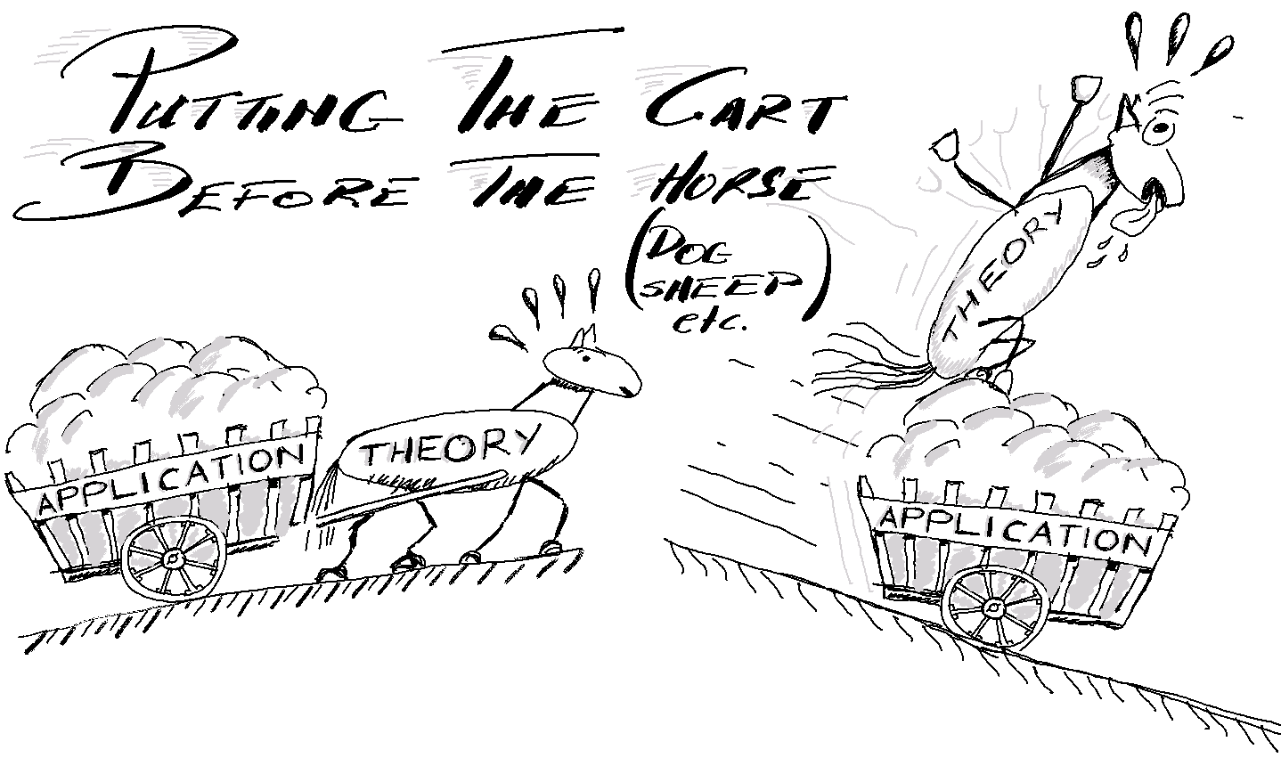
Figure 0.1: Most scientific disciplines proceed by developing theoretical constructs and testing them against the real world. Once some confidence has been gained that these can capture some aspects of reality, they are used to guide applications. However, when the urgency of the applications is high, as is often the case with contemporary conservation and environmental problems, the use of methods can overtake our understanding of them. This certainly feels true about the literature linking species to their habitats, where we are often not sure how to interpret the inputs, structure and outputs of our statistical models.
0.5 Why is this book unique?
By drawing parallels and intersections between plants and animals, the material presented here tries to unify our conceptual and methodological approach to SHAs across living taxa. By doing so, we hope to generate some cross-fertilization between the disparate analytical approaches traditionally used to investigate the distribution and habitat preferences of sessile and mobile species. Indeed, we aim to extend movement-related models and habitat selection concepts that are usually associated solely with animals to plant movement and selection over longer time scales, between life-stages, between generations, or even across different morphs along the evolutionary timeline.
We also try to achieve unification across scales. Species distributions are dynamic and spatially structured, but the data we collect often cover a specific spatial region or time window. For example, tracking an animal moving within a well-defined home-range, may tell us something about the behavior and resource selection of that individual, but may not be informative about how that animal established its home range there. Alternatively, using museum records, we may look into the distant past, and capture global distributions, but these distributions may not help us understand fine-scale selection, and they may also not match the current distribution of a species following recent anthropogenic change. To address these issues, we need to consider hierarchical spatial models that allow for non-equilibrium dynamics.
This book also tries to achieve convergence between existing statistical methodologies. Our feeling is that the literature currently comprises many methods that are already well connected, a few methods that represent analytical dead-ends and several methods that merely appear isolated and are waiting to be linked to our main body of work via re-interpretation. Hence, rather than offer a mixed bag of quantitative recipes, we have selected available and emerging methods that we feel combine into a coherent and expandable framework.
Finally, we try to achieve unification of modeling paradigms by bringing together mathematically formulated mechanisms with the statistical machinery needed for extracting information from field data. For example, classic mechanistic models from the 1970s, such as the ideal free distribution (Fretwell & Lucas, 1969), have connected environmental productivity with species distribution by considering the behavior of ideal individuals (Křivan, Cressman, & Schneider, 2008). In more recent years, flexibility in species-habitat association models has come from statistical approaches, like generalized additive models (Wood, 2006) using smooth functions of covariates, whose constraints are data-driven. We can gain much by replacing the extremely flexible smooth functions with pre-defined dependencies between the organism and the environment, e.g. by motivating the functional forms of models from biological first principles, or by including informative priors for some of our model parameters.
0.6 Why model species habitat associations?
There are many specific reasons why ecologists are interested in developing SHA models, but, in their essence, these can be split into three broad categories. Given a sample of spatial observations from a species (or a population, a social group, or even a single individual) together with environmental data from the same region in space and time period, we aim to quantify: 1. where organisms occur (spatial estimation); 2. why they occur there (inference); 3. where else they might occur (prediction); There is a clear ramp-up in difficulty in these questions. In its simplest form, spatial estimation is purely pattern-based whereas prediction (in space or time) arguably requires deeper insights into behavioral, energetic, demographic and community mechanisms.
0.6.1 Spatial estimation
Spatial estimation or ‘map-making’ could be achieved by means of density estimation methods, using only the spatial coordinates of observed locations [e.g., various smoothing approaches such as kernel or spline methods; Silverman (1986)]. Species distribution maps can be valuable for conservation and population management purposes. For instance, by highlighting where certain (rare) species occur, they can assist in the designation of protected areas (Moilanen, Wilson, & Possingham, 2008). Maps can also be used to quantify the impact of anthropogenic activities on wildlife by estimating direct encounters (e.g., collisions of birds with wind turbines, wildlife-vehicle collisions along road networks, bycatch of seabirds or marine mammals in longlines and fishing nets), or sub-lethal effects (e.g. impact of military sonars on marine mammals, exclusion of foragers from valuable food sources, alteration of migration routes due to climate change). Potentially, maps can be used by ecologists as stepping-stones for further analysis. E.g., when studying predator-prey interactions, a previously estimated density map of prey could be used as an explanatory variable for the distribution of the predator.
0.6.2 Inference
For the second aim of understanding why certain organisms occur where we observe them, a relationship needs to be established between the distribution of organisms and relevant environmental variables that surround the organisms. For example, plant distribution modeling may be used to quantify the temperature or soil pH ranges within which the study species occur, or to investigate their tolerance for extreme events, like droughts or inundation (Sarker, Reeve, Thompson, Paul, & Matthiopoulos, 2016). This has led plant ecologists to think primarily in terms of physiological tolerances, and environmental envelopes (Pearson & Dawson, 2003). In contrast, animal ecologists use selection functions, such as Resource-Selection Functions (Boyce & McDonald, 1999) or Step-Selection Functions (Thurfjell, Ciuti, & Boyce, 2014) to quantify which combinations of environmental attributes animals select from a list of available options. These models provide insights into why and how animals migrate (McClintock et al., 2012; Börger et al., 2013), what drives the distribution of their breeding sites (e.g. in colonial marine predators) (Robinson et al., 2017), and possible symbiotic (or exclusion) effects between species (Ovaskainen & Abrego, 2020).
0.6.3 Prediction
The third aim, predicting species distributions in space and time (Elith & Leathwick, 2009), is probably the most challenging, and the most reliant on the successful completion of prior steps (i.e. a good model fit to observed density using sufficiently insightful environmental variables). Applications related to prediction are targeted at vital questions, such as species range expansion or contraction (Scheele, Foster, Banks, & Lindenmayer, 2017), risk assessment for invasive species (Gallien, Douzet, Pratte, Zimmermann, & Thuiller, 2012), recovery after temporary displacement (Russell et al., 2016), and redistribution following permanent displacement (Street et al., 2015), as well as classic questions regarding impacts of habitat destruction or fragmentation due to human infrastructure development (Beyer et al., 2016). All of these apparently divergent questions are driven by a desire to have models that are transferable to novel environments in space or time (Yates et al., 2018) - i.e. we want our models to give robust predictions even when they are ripped out of the spatiotemporal context in which they were trained. For ecologists, obtaining robust predictions under-change is a primary objective. However, most available statistical methods focus on association rather than causal inference, and rely on environmental explanatory variables that are most readily available, rather than have a causal relationship with the species’ ecology. Further, we tend to evaluate models based on goodness-of-fit rather than their predictive capacity (Fourcade, Besnard, & Secondi, 2018). As we illustrate throughout this book, the pragmatic resolution of such dilemmas for real-world applications centers around enhancing the mechanistic content of our statistical models.