Chapter 2 Modelling Species-Habitat Associations
2.1 Objectives
The objectives of this chapter are to:
Explore the function and scope of the process component of a Species Habitat Association Model. How can we translate basic ecology into basic models?
Outline the two necessary ingredients of process models for species-habitat associations: the availability of habitats in the environment and their resulting usage by animals, or plants.
Present the Use-Availability (U-A) approach, a broad conceptual framework that encompasses all existing SHA process models and can be expanded to incorporate more biological realism.
Introduce the connection between U-A models fitted in environmental space (E-space) and the expected usage surfaces mapped in geographical space (G-space).
Explain how the structure of the process model can describe responses to resources, conditions and risks, capture trade-offs and complementarities between resources.
Suggest future extensions to process models that are not currently implemented in published studies, but are anticipated by theoretical models.
2.2 You are here
This chapter focuses on how the biological questions and challenges from Chapter 1 can be formalized into expandable mathematical frameworks. To link up with the biological motivation of SHAs, the underlying frameworks seek to address questions about individual selection (a behavioral process) and state (a physiological and life history process). They also aspire to be relevant to predictions about population viability and demographic functions. These biological motives are best satisfied in environmental (or niche) space. However, this chapter also aims to link forward to Chapter 3, by translating the predictions of environmental models into observable, geographical space. The first three chapters together, achieve the transition from questions-to-data and back again.
2.3 Formalising the association between habitat and species
The most common image conjured up when considering species-habitat associations is of several spatial layers of environmental variables being fed into a statistical model, that produces (often, with a considerable degree of automation) a corresponding species layer (Fig. 2.1). This output layer is thought of as representing some notion of habitat suitability, or expected usage.
Within the SHA community, this kind of representation (a glorious sandwich of geographical layers achieved by a statistical model) has immense appeal for five reasons. First, geographical space is intuitive. It is, after all, the natural space that we inhabit, we perceive, and have built intuition in. Second, animals and plants give us evidence of their preferences for particular habitats by coinciding spatially with those habitats. Third, statistical models are simple, quantitative and sufficiently removed from biological mechanism. This makes them objective (a good thing) and, at the same time, almost immune to biological criticism (a really bad thing). Fourth, color maps of habitat suitability are intrinsically beguiling and often difficult to dispute, especially when the quantity they depict is not defined precisely. Finally, the geographical viewpoint is partly a historical relic from earlier times when studies did not use statistical models, but just visually compared different GIS layers. All these sources of appeal (to which we must also admit our own vulnerability), have made the SDM workflow appear understandable and, even, trivial.
There is little doubt that we need to (somehow) funnel the influence of multiple environmental variables into a single map representing habitat suitability, so the general notion of Fig. 2.1 is correct, but its implementation into models conceals two pitfalls. As the users and developers of these methods, we need to consider exactly how the input layers (let us call them \(x_1, x_2, x_3, ...\)) are combined within the model’s black box, and we also need to define, precisely, the meaning of the model’s output.
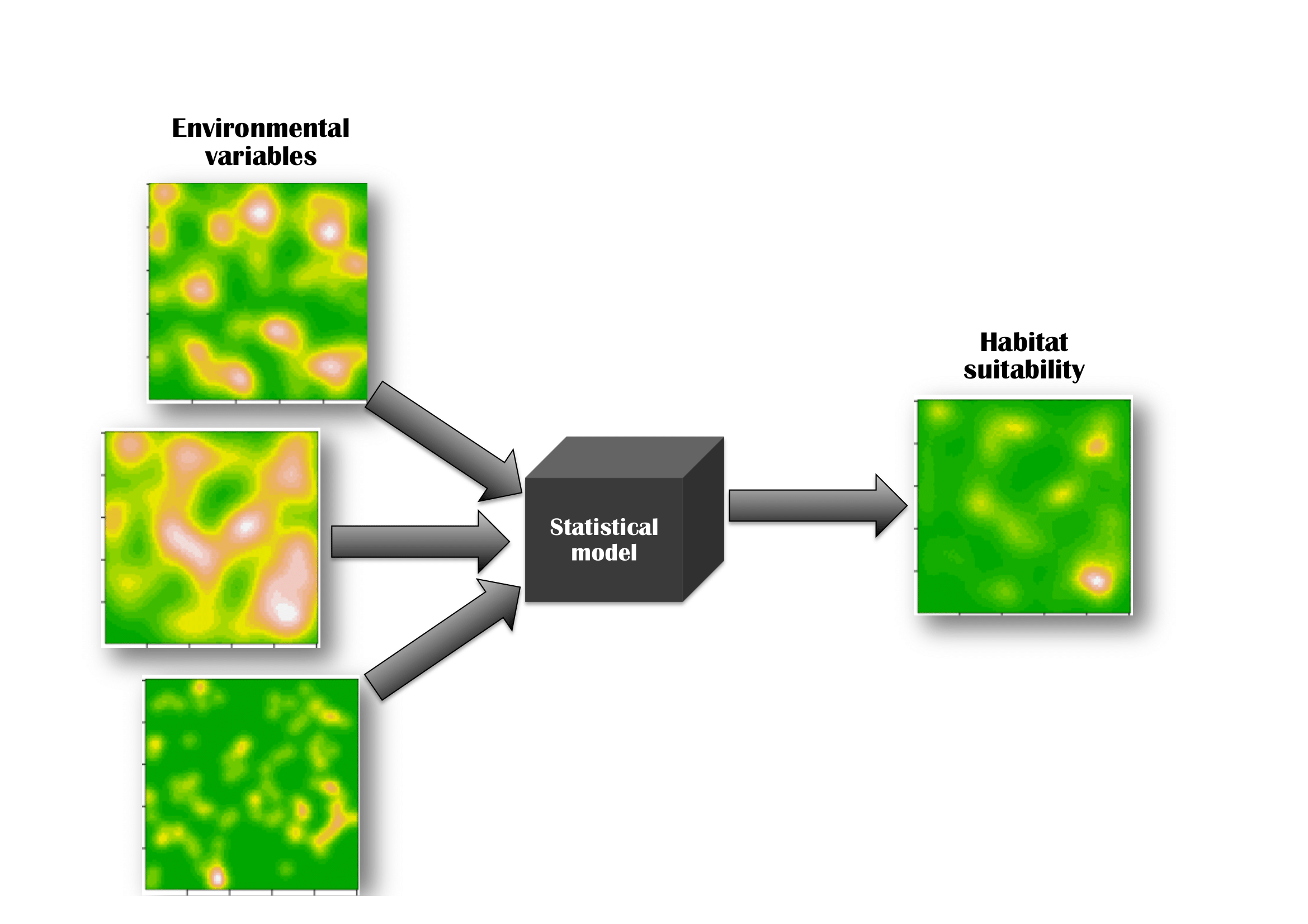
Figure 2.1: Species-habitat association models are usually imagined in geographical space as a superposition (a combination) of environmental layers, into some measure of habitat suitability, via a statistical model. The statistical model is often treated as a black box, and the emphasis is placed on the relative contribution of the input layers to the resulting map.
The exact mathematical translation of Fig. 2.1 is the addition of multiple layers into a single, resultant map. Then, each cell of the output layer would be calculated by the corresponding values (\(x_1, x_2, x_3, ...\)) of the cells of the input layers
\[\begin{equation} \sum_{k=1}^K{x_i}=x_1+x_2+...+x_K \tag{2.1} \end{equation}\]
Of course, not all inputs are equally important for the resultant (however we choose to define this resultant, biologically), so we should allow for the possibility of adjusting the contribution of the different layers according to some coefficients \(\alpha\). Something like
\[\begin{equation} \sum_{k=1}^K{\alpha_k x_k}=\alpha_1 x_1+\alpha_2 x_2+...+\alpha_K x_K \tag{2.2} \end{equation}\]
If we impose no constraints on the sign and value of these coefficients and input layers, this kind of expression can take any values between \(-\infty\) to \(+\infty\), which is not ideal, if we want to use it to describe things like expected usage (a non-negative quantity). So, we may need to constrain this expression in an appropriate way, depending on the definition of the output layer.
More challenges like these soon present themselves. For example, there is nothing to say that such additive combinations of the inputs are realistic. As we saw in Chapter 1, environmental variables can act in ways that are highly non-linear. Trade-offs, synergies, complementarities between variables are the biological rule, not the exception in how the environment affects the distribution of species. Also, when asking population-level questions, how can we account for the fact that individual animals and plants can behave in different ways in different contexts and during different life-history stages? How can we account for population composition, density-dependent processes and evolutionary pressures?
If we think biologically about these problems (as we always should), then suddenly, the simplistic, phenomenological approach of Fig. 2.1, seems very far away from the questions we are trying to answer with it. How do we attempt to move from pattern-driven (phenomenological) models, to process-based (mechanistic) ones?
The process component of a SHA model is ultimately intended to encapsulate all of the ecological truths that can be feasibly extracted from the available data via the process of model fitting (see Chapter 3). Ideally therefore, the parameters built into the process model should be biologically interpretable. In theory, a fully-detailed process model should be able to inform us about the behavioral decisions mediating habitat selection, the energetic and nutritional trade-offs and synergies of resources on animals and plants, the effect of conspecifics and heterospecifics on the expected distribution of usage, etc. However, the degree to which process parameters are amenable to interpretation depends on how mechanistically-motivated a process model is. Traditionally, research in this area has tended to think of SHA process models as purely phenomenological (e.g. Generalized Linear Models - GLMs), and has attempted to catch glimpses of biological causality by observing the direction and magnitude of correlations between usage and its suspected covariates. Have a look at eq. (2.2), which already looks like the linear predictor of a GLM. The parameters \(\alpha_i\) are a far-cry from basic biological parameters with clear physical interpretation (such as an individual’s basal metabolic rate or the handling time needed to consume its prey).
However, the underlying process framework need not be constrained solely to providing such indirect inferences. For many years, we have had access to process models with high levels of biological detail (Nisbet & Gurney, 2004; Otto & Day, 2011; Murray, 2013), and recently, we have been acquiring the statistical ability to confront them with field data (Newman et al., 2014; Hooten, Johnson, Mcclintock, & Morales, 2017; Kery & Royle, 2020). A good strategy, when approaching the empiricism-mechanism dilemma, is to start with an empirical model that can be incrementally (and strategically) expanded with mechanistic detail. Therefore, in this chapter, we take the broadest possible view of process models in SHAs, aiming to embed simple phenomenological models in their true context and, also, to signpost the routes that can be followed to flesh-out these skeleton empirical models with more biological mechanism.
2.4 The meaning of the SHA model output
So, how should we interpret the output of the SHA process model? There are a great many options to choose from, unfortunately, and not all of them are correct for particular process models. For example, for most currently available models, the interpretation of the output as a measure of habitat suitability is more wishful thinking than truth. As we explained in Chapter 1, organisms are frequently found at places that are not suitable for them (e.g. either because they have to transit through them, or because they overflow from nearby suitable places). Conversely, organisms are frequently not found at places that may be suitable for them (e.g. either because they have not yet extended their range to include these places, or because they need complementary access to other habitats, that happen not to be nearby). Various flavors of “niche-related” models (A. H. Hirzel, Hausser, Chessel, Perrin, & Jul, 2002; Alexandre H. Hirzel & Le Lay, 2008; Broennimann et al., 2012; Robertson;, Caithness, & Villet, 2012) assume that population density is proportional to fitness. This presumption will influence the biological conclusions to an unknown extent (Peterson et al., 2011). In Chapter 1, we introduced a null model for SHAs that preserved the correspondence between distribution and fitness, precisely to allow us to discuss and develop the main ideas of SHAs without worrying about these additional biological complications. We will return to these problems (and proposed solutions) repeatedly in this book, but for now, we need a working definition of the model output.
The final output of a SHA process model represents expected spatial usage by an individual or a population
Here, we use the term expectation in its statistical sense (as a population mean or long-term average). Spatial usage may be defined as a relative measure, a proportion attributed to each cell in geographical space, or a probability density associated with each set of spatial coordinates. Alternatively, in the case of entire populations, usage may be defined as an absolute amount, integrating to the total population size, over the whole of space.
2.5 The process model, as a black box: Inputs and outputs
We begin by considering the inputs and outputs of a SHA model, particularly focusing on their constraints. In general, the process model can be thought of as a function \(h\) that takes input values from a domain \(\mathbb{X}\) and gives output values in a range \(\mathbb{U}\).
\[\begin{equation} U=h(\mathbf{x})\hspace{20mm} h:\mathbb{X}\to{\mathbb{U}} \end{equation}\]
The domain, range and structure of the mathematical model can vary in their definition and complexity. If we consider the process model as a black box operating on its input(s), to produce its output(s), the possible definitions of the domain and range can be quite informative.
For example, the domain \(\mathbb{X}\) can be thought of environmentally, spatially and temporally. A spatial domain \(\mathbb{G}\), or G-space may be defined in terms of latitude and longitude on a map (with the possible addition of altitude, or sea-depth as a third spatial dimension). Any subset of G-space is possible (e.g. resulting from the boundary of a particular study region). An environmental domain \(\mathbb{E}\), or E-space may be defined in terms of continuous or discrete environmental variables. Examples of continuous variables include temperature, humidity, food abundance, predator abundance etc. Examples of discrete variables include pre-designed classifications of the environment into habitat classes (as is often done for the purposes of preparing color maps by Geographic Information Systems). A temporal domain \(\mathbb{T}\), or T-space is defined as any subset of the real numbers signifying a time interval. Most SHA models are defined in \(E\)-space (so that, \(\mathbb{X}=\mathbb{E}\)). All purely spatial models (e.g. most geo-statistical or trend-fitting models) are defined in \(G\)-space (so that, \(\mathbb{X}=\mathbb{G}\)).
Combinations of those spaces are, of course, possible and there are some examples (Hedley & Buckland, 2004; Augustin, Trenkel, Wood, & Lorance, 2013) of habitat models that account for residual spatial autocorrelation by using spatial dimensions (so that, \(\mathbb{X}=\mathbb{E}\cup\mathbb{G}\)). Such models effectively fold the spatial location into the definition of “habitat” (making each location a unique habitat, and each habitat a unique location). Such geographical extensions of the process model are made mostly as heuristic tools to increase the variability explained by SHA models and, on some occasions, they can motivate ideas about the shape of missing covariates.
The temporal dimension is occasionally employed to augment the domain (\(\mathbb{X}=\mathbb{E}\cup\mathbb{T}\)), leading to the construction of dynamical SHA models (Augustin et al., 2013; Hooten, Hanks, Johnson, & Alldredge, 2014).
| Domain (\(\mathbb{X}\)) | Examples |
|---|---|
| \(\mathbb{E}\) | Species association with food and water |
| \(\mathbb{G}\) | Description of a spatial trend in species density |
| \(\mathbb{E}\cup\mathbb{G}\) | A species invasion gradient interacting with habitat variables |
| \(\mathbb{E}\cup\mathbb{T}\) | Seasonality in habitat responses |
| \(\mathbb{G}\cup\mathbb{T}\) | A dynamic gradient in space |
| \(\mathbb{E}\cup\mathbb{G}\cup\mathbb{T}\) | Seasonal responses to habitat on a multi-annual invasion gradient |
Table 2.1, shows some increasingly fanciful possibilities of process model domains, but for much of this book, we will consider SHA models fitted exclusively in E-space. Although we may occasionally consider spatial proximity between habitats, we will not usually employ the specific location within the process model.
The process model associates a value of absolute or relative usage, with each point in the model’s domain (see Section 2.4). Therefore, for the vast majority of SHA models, the range \(\mathbb{U}\) of values is assumed to be one-dimensional. Indeed, with no loss of generality, we can think of the output (the relative usage of any given habitat \(\mathbf{x}\)) as a proportion of an individual’s time or the portion of a whole population, so that so that, \(\mathbb{U}=[0,1]\). Conceivably, it is possible to extend our process model’s range to multiple dimensions. Such models could, for example, simultaneously look at the associations of multiple species with habitat (Guisan & Zimmermann, 2000; Ovaskainen, Hottola, & Shtonen, 2010; Wisz et al., 2013; Ovaskainen & Abrego, 2020).
2.6 Usage in Geographical and Environmental spaces: Model transferability
Let us consider the example of two environmental variables that act as resources for a particular species. In Figs 2.2a,b we show two such examples plotted in G-space. We assume that the organism can aggregate its usage in regions of space that offer a good combination of both resources (according to some unknown preference function, expressed by the organism through some unknown selection process). This behavior gives rise to a utilization distribution shown in Fig. 2.2c. The colors in that figure represent the frequency of use of a particular location \(\mathbf{s}\) in geographical space (dark greens for low usage and light browns for high).
However, most of our SHA models are not designed to be explicitly spatial, for one very good reason to do with model transferability. A model that is formulated to produce predictions about particular points in space \(\mathbf{s}\) is only directly usable for prediction if we are interested specifically in those points3. In contrast, a model that anticipates usage of a particular habitat \(\mathbf{x}\) has the potential to give us useful predictions for times and places other than those for which we have data. Achieving transferability in predictions is the holy grail of SHA models (Randin et al., 2006; Tuanmu et al., 2011; Wenger & Olden, 2012; Sequeira, Bouchet, Yates, Mengersen, & Caley, 2018; Yates et al., 2018; Qiao et al., 2019), and a core theme of this book. Although this highly desirable property cannot be achieved simply by thinking and modeling in E-spaces, doing so is a prerequisite for transferable SHA models.
It therefore helps to be able to think of biological processes in E-spaces, i.e. spaces whose dimensions are environmental variables, rather than geographical coordinates. In principle, they are more challenging to visualize because they can very easily become high-dimensional (no ecological system exists in more than three geographical dimensions, but most systems are usually influenced by a myriad of environmental variables). However, thinking about E-spaces in one or two dimensions (i.e. in terms of one or two environmental variables) builds intuition that is readily transferable to more complex, multidimensional E-spaces. Plotting the observed usage of G-space (Fig. 2.2c) in E-space, requires us to identify all G-cells that are characterized by similar combinations of resources, and to sum the proportions of usage they contain. We will use the symbol \(f\) to denote frequencies plotted in this way in E-space. Since each cell in this plot represents the frequency of usage of a habitat \(\mathbf{x}\), we will denote this quantity by \(f_{u}(\mathbf{x})\).
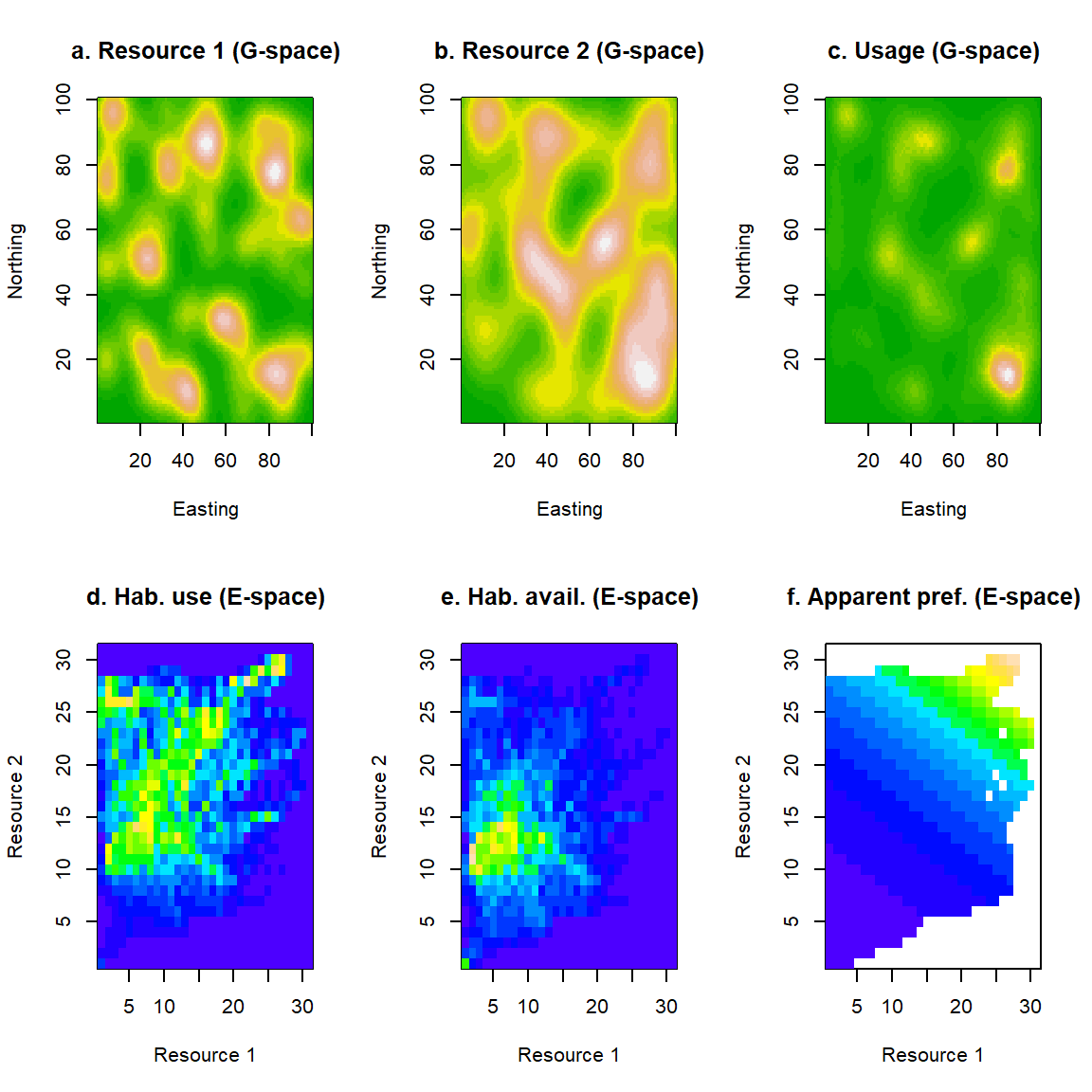
Figure 2.2: An example of use and availability of habitats in geographical and environmental space. We consider two geographical layers (a and b) representing the geographical distribution of two resources. On those, we superimpose the utilisation distribution (c) of a hypothetical animal. We can recast this information into environmental space. Usage of habitats in E-space (d) is, essentially, a histogram of the frequency with which different resource combinations are used by the animal. Similarly, the availability of habitats in E-space (e) is the frequency with which different combinations of resource abundances occur in the environment. A measure of apparent habitat preference (f) can be obtained by dividing habitat use (d) by habitat availability (e). Here, white space indicates division by zero (i.e. non-existent habitats).
The result is shown in Fig. 2.2d, plotted in a different color scheme, to emphasize the transition from G- to E-space. Cells close to the origin of this plot represent habitats that are low in both resources, whereas habitats towards the top right corner represent utopian habitats with an embarrassment of riches. In that map, cold blue colors represent lack of usage, whereas warmer colors (towards yellow) show us habitats that are used a lot. As might be expected, the habitats at the bottom-left of E-space are not used very much, but, perhaps less intuitively, the utopian habitats at the top right are not used at all. What is going on?
2.7 Lifting the black box lid: Habitat usage and habitat availability
Well, the answer becomes easy to guess if, instead of usage, we focus on visualizing habitat availability in E-space (Fig. 2.2e). This new quantity, let us call it \(f_{a}(\mathbf{x})\), represents the frequency with which habitats of similar characteristics appear in the environment at-large. Notice the dark blue colors at the top-right of that plot: Utopian habitats do not physically exist, which might explain why they appear not to be used in Fig. 2.2d. The pattern of apparent habitat preference, is better revealed in Fig. 2.2f, where we have attempted to control for the effects of habitat availability by plotting the ratio of usage over availability \(f_{u}(\mathbf{x})/f_{a}(\mathbf{x})\). The white areas of this plot are essentially non-existent habitat, so the picture is not strictly complete, however, the colored areas reveal a very simple tendency in habitat preferences of “more-is-better”, as the color gradient goes diagonally from low (bottom-left) to high (top-right).
Quantifying the availability of a habitat is an essential part of any attempt to quantify preference for that habitat (D. H. Johnson, 1980). It is generally impossible to express total usage of a habitat purely as a function of preference (Jason Matthiopoulos, 2003a) because doing so would imply that organisms can use habitats that do not physically exist. If this point seems self-evident, then perhaps it is valuable to highlight that there are several methods that make just this assumption (A. H. Hirzel et al., 2002; Broennimann et al., 2012; Robertson; et al., 2012).
Fig. 2.2 also reveals another common truth about G- and E-spaces. In general, objects in G-space are more likely to have multiple peaks and troughs, since there may be several different areas in G-space with similar properties. Indeed, the whole part of the ecological literature that deals with patchy environments and metapopulation occupancy patterns, is a direct result of that fact. However, E-space gradients in habitat availability, usage and especially preference, are comparatively simpler constructs, that are more easily captured by monotonic, or unimodal mathematical models (Jason Matthiopoulos et al., 2020). If you cast your mind back to our classification of environmental variables from Chapter 1, in theory, the behavior of habitat preference along any single dimension of E-space can be modeled as an increasing (resource), decreasing (risk), or unimodal (condition) function.
With all of the above in the background, it appears that to understand species-habitat associations, we need to consider habitat availability, because what an organism will be observed using depends on what it needs/wants and what it can find/access. We want to ensure that observed usage will be zero both for undesirable and for unavailable habitats (2.3).

Figure 2.3: Use of space by organisms, is a combination between two influences. What kinds of habitats they prefer (or, can survive in) and what kinds of habitats are available to them. Habitats may be unavailable either because they don’t exist, or because they are not accessible.
Multiplication is a good trick here4:
\[\begin{equation} \text{What I use}=(\text{What I want})\times(\text{What I can find}) \end{equation}\]
The underlying biology of these loosely used words is considerable. The choices of organisms are not necessarily fully expressed by them within the frames of observation, or in a way that is always aligned with their fitness. Similarly, the availability of habitats to organisms relies on a complex interplay between landscape structuring, organisms’ cognition and mobility (Jason Matthiopoulos, 2003b; Jason Matthiopoulos et al., 2020). Be that as it may, if we pretend for the moment that we have some intuitive understanding of these concepts, we can plausibly write the expected usage of a habitat in terms of some function \((h)\) expressing habitat preference
\[\begin{equation} f_{u}(\mathbf{x})=h(\ )f_{a}(\mathbf{x}) \tag{2.3} \end{equation}\]
The function \(h()\) is the core of the process model and will ultimately be required to absorb all the intricate biological mechanisms described in Chapter 1. So, how do we start giving it a form? Biologically, the simplest version of the function \(h\) is constant, implying that an organism will use a habitat in proportion to its availability.
\[\begin{equation} f_{u}(\mathbf{x})=hf_{a}(\mathbf{x}) \end{equation}\]
Indeed, if usage and availability are expressed as density functions (such that, \(\int_{\mathbb{E}}{f_{u}(\mathbf{x})d\mathbf{x}}=1\) and \(\int_{\mathbb{E}}{f_{a}(\mathbf{x})d\mathbf{x}}=1\)), then the proportionality relation implies that usage is equal to habitat availability (i.e. \(h=1\)). The biological scenarios that justify this kind of model are restricted to indiscriminate organisms, species that roam the entire landscape without preferentially selecting to move to, or even linger in, some habitats over others. Arguably, from the point of view of species-habitat association, this model is somewhat boring, because it implies no association at all. It is nevertheless, an appropriate null model for the process of selection, because it corresponds to uniform usage of G-space.
Deviations from this null model, are thought of as manifesting disproportionate usage of habitats compared to their availability. This is the point where we can start talking about habitat selection. Mathematically, we can achieve this behavior by writing \(h\) as a function of habitat.
\[\begin{equation} f_{u}(\mathbf{x})=h(\mathbf{x})f_{a}(\mathbf{x}) \tag{2.4} \end{equation}\]
Regarding the properties of \(h(\mathbf{x})\), we know that it needs to be non-negative because it makes no sense to define a multiplier for availability that may lead to negative usage. We also know that it must preserve the unit-sum properties of usage because no individual or population can exist for more (or less) than 100% of their time in this world (i.e. \(\int_{\mathbb{E}}{f_u(\mathbf{x})d\mathbf{x}}=1\)). Therefore, we need:
\[\begin{equation} h(\mathbf{x})\geq0 \ \ \ ,\ \ \ \int_{\mathbb{E}}{h(\mathbf{x})f_a(\mathbf{x})d\mathbf{x}}=1 \tag{2.5} \end{equation}\]
In this first model of disproportionate usage, we can rewrite eq. (2.4) as
\[\begin{equation} h(\mathbf{x})=\frac{f_{u}(\mathbf{x})}{f_{a}(\mathbf{x})} \tag{2.6} \end{equation}\]
which gives us an intuitive model for the habitat preference function, as the ratio of a habitat’s usage over its availability. If you need to visualize this, then just look at the example of Fig. 2.2f, which shows exactly this ratio across E-space.
2.8 Thinking inside the box: Mathematical formulations
Now, let us try and put some more details into our definition of the process model. We will do this incrementally, leading up to a correct expression for \(h(\mathbf{x})\). Let us imagine that we want to write habitat preference as some simple linear combination \(g(\mathbf{x})\) of the characteristics of a habitat. This follows the superposition rationale from Section 2.3, and, in particular, eq. (2.2). In general, for a vector of \(n\) environmental variables \(\mathbf{x}=(x_1,...,x_K)\) this could be
\[\begin{equation} g(\mathbf{x})=\sum_{k=1}^K{a_k x_k} \tag{2.7} \end{equation}\]
We will call \(g(\mathbf{x})\) the predictor function, a name that echoes the linear predictor functions of GLMs, but still allows a potential relaxation of linearity, in more elaborate models. For the simple example of habitat preference with two resources, seen in Fig. 2.2, the predictor function was
\[\begin{equation} g(\mathbf{x})=0.04x_1+0.08x_2 \end{equation}\]
In this example, we had positive coefficients in response to both environmental variables but, in many cases (e.g. environmental risks), we might like to express avoidance for increasing values of an environmental variable. In these cases, the coefficients of the model may need to take negative values, and ultimately yield negative values overall for the preference function. This is expressly forbidden by eq. (2.5) which requires a non-negative valued function. There are many ways that an unbounded expression can be constrained to be non-negative (e.g. by taking its absolute value or raising it to an even power). The SHA literature customarily uses the exponential function. We will denote this transformed predictor function by \(w(\mathbf{x})\)
\[\begin{equation} w(\mathbf{x})=exp(g(\mathbf{x})) \tag{2.8} \end{equation}\]
We will call \(w(\mathbf{x})\) the resource (or habitat) selection function, a well-established name for this function (Boyce & McDonald, 1999; Mark S.Boyce, Pierre R.Vernier, Scott E.Nielsen, & Fiona K.A.Schmiegelow, 2002). Although this ticks the positivity requirement for eq. (2.5), we still need to ensure that its second (unit-sum) requirement is observed. For example, as the values of \(x_1\) and \(x_2\) become larger across a landscape, there is nothing to stop eq. (2.8) from integrating to more than one. We can put a cap to that value by normalizing, as follows:
\[\begin{equation} h(\mathbf{x})=\frac{w(\mathbf{x})}{\int_\mathbb{E}{w(\mathbf{x})f_a(\mathbf{x})d\mathbf{x}}} \tag{2.9} \end{equation}\]
Alternative ways of writing the function \(h\) are
\[\begin{equation} h(\mathbf{x})\propto w(\mathbf{x}) \ \ \ \ or \ \ \ h(\mathbf{x})=k^{-1} w(\mathbf{x}) \tag{2.10} \end{equation}\]
where
\[\begin{equation} k=\int_\mathbb{E}{w(\mathbf{x})f_a(\mathbf{x})d\mathbf{x}} \tag{2.11} \end{equation}\]
The proportionality constant \(k^{-1}\) is needed if we want to eventually attach some numbers to the above symbols. Considering the value of \(k\) in detail is relatively unimportant for following the main thread of the story here, but it does hide a valuable story of its own. Calculating \(k\) from eq. (2.11) requires us to consider the relative response of organisms to all relevant habitats. This means that, ultimately, any quantification of the usage, or preference of a particular habitat, cannot be achieved without consideration of the usages and preferences of all accessible habitats in the environment of an organism. In other words, it doesn’t matter how large the value of the selection function \(w(\mathbf{x})\) is for a particular habitat \(\mathbf{x}\), what matters is how much larger that value is compared to all other habitats.
We have so far presented three useful functions. The preference function \(h(\mathbf{x})\), the selection function, \(w(\mathbf{x})\), and the predictor function \(g(\mathbf{x})\). These are nested within each-other as follows:
\[\begin{equation} h(w(g(\mathbf{x})))=\frac{exp(g(\mathbf{x}))}{\int_\mathbb{E}{exp(g(\mathbf{x}))f_a(\mathbf{x})d\mathbf{x}}} \tag{2.12} \end{equation}\]
Bringing eq. (2.9) together with eq. (2.4) gives a complete expression for habitat use.
\[\begin{equation} f_u(\mathbf{x}) = \frac{w(\mathbf{x})f_a(\mathbf{x})}{\int_{\mathbb{E}} w(\mathbf{z})f_a(\mathbf{z}) d\mathbf{z}} \tag{2.13} \end{equation}\]
Later, in section 3.5, we will see how this expression is employed by weighted distribution theory (Subhash R. Lele, 2009) to fit these models to data.
2.9 Spatial intensity from habitat preference
The development and interpretation of SHA models requires some familiarization with G- and E-spaces. We need to be able to move from physical to niche space and back again. In section 2.6, we made the forward transition (G- to E-space). In this section, we discuss how to go back. To visualize our predictions in G-space, we need a notion of usage per unit area of habitat. Let us consider the example of a species, observed in a completely synoptic way (i.e. all occurrences of every individual in the population are recorded). A total of 1000 observations are made. A total of 120 observations are recorded in a particular type of habitat. Taking a look at the map of the study area, we measure that the total area occupied by this habitat is 3000\(m^2\). Therefore, the average number of observations (from our total sample of 1000) to be found in each \(m^2\) of that habitat will be \(\frac{120}{3000}=0.04\). In general, therefore
\[\begin{equation} \text{Usage per unit area of habitat }\mathbf{x}=\frac{\text{Total usage of habitat }\mathbf{x}}{\text{Total area of habitat }\mathbf{x}} \end{equation}\]
The proportion of usage of this population to be found in any one \(m^2\) belonging to that particular habitat will be \(\frac{0.04}{1000}=4\times 10^{-5}\). Generating this kind of (per-unit-area) calculation for every habitat type can allow us to populate each cell in G-space with values, leading to a map of expected usage by an individual, or a population.
Assuming that we have obtained functions for habitat use and availability in E-space, can we construct a per-unit-area calculation for plotting G-space maps? The trick is to look at the definition of habitat preference from eq. (2.6):
\[ h(\mathbf{x})=\frac{f_{u}(\mathbf{x})}{f_{a}(\mathbf{x})} \]
We can expand each of the three quantities in this expression. From eq. (2.10), we have
\[ h(\mathbf{x})=k^{-1} w(\mathbf{x}) \]
From the definitions of \(f_{u}(\mathbf{x})\) and \(f_{a}(\mathbf{x})\) as probability functions, we can write:
\[\begin{equation} f_{u}(\mathbf{x})=\frac{\text{Total usage of habitat } \mathbf{x}}{\text{Total usage of space}} \end{equation}\]
\[\begin{equation} f_{a}(\mathbf{x})=\frac{\text{Total area of habitat } \mathbf{x}}{\text{Total area of space}} \end{equation}\]
Since \(k\), the total usage of space and the total area of space are constants across some subset of geographical space (say, our study region), we can rewrite eq. (2.6) as
\[\begin{equation} w(\mathbf{x})\propto\frac{\text{Total usage of habitat }\mathbf{x}}{\text{Total area of habitat }\mathbf{x}} \end{equation}\]
Therefore, \(w(\mathbf{x})\), as given in eq. (2.8), is proportional to the use of a cell of type \(\mathbf{x}\) in G-space. We will use \(\lambda(\mathbf{s})\) to denote the expected usage at a geographic location \(\mathbf{s}\). This gives us the fundamental relationship between E-space and G-space.
\[\begin{equation} \lambda(\mathbf{s})\propto w(\mathbf{x}(\mathbf{s})) \tag{2.14} \end{equation}\]
The expected usage of a geographical location (\(\mathbf{s}\)) is proportional to the value of the selection function associate with the habitat characteristics at that location (\(\mathbf{x}(\mathbf{s})\)). Eq. (2.14) also delivers a simple algorithm for generating spatial maps of expected usage from a SHA model. Here are the steps:
- Consider any spatial location \(\mathbf{s}\) in G-space
- Take the vector of habitat characteristics \(\mathbf{x}(\mathbf{s})\) at the coordinates of that location
- Express the value of the resource-selection function \(w(\mathbf{x}(\mathbf{s}))\)
- Assign that value to the location \(\mathbf{s}\)
- Repeat for all locations in G-space
- Normalize all the values so that they add up to 1 (i.e. 100% of usage) for the whole of space
For example, consider the maps of two resources (say \(x_1\) and \(x_2\)) in G-space. Let us assume that these maps are matrices5 and have the same dimensions. Let us further assume that the RSF for this species is given, simply, by:
\[\begin{equation} w(\mathbf{x})=e^{0.04x_1+0.08x_2} \end{equation}\]
The R-code to plot a map of lambda would be:
w<-exp(0.04*x1+0.08*x2)
lambda<-w/sum(w)
image(lambda)
There is one feature of G-space that can wreak havoc on spatial predictions. We will call this accessibility for short and will come to define it more clearly in section 3.11.2. Consider the following biological examples where the transition from E- to G-space may give unrealistic maps:
We are interested in the distribution of usage of a particular pack of wolves who constrain their use of space to their home range, a subset of the landscape. Hence, not all of space is accessible to them and if we apply the above approach indiscriminately on all of the landscape, we will be spreading the pack’s fixed amount of usage rather thinly, hence overestimating the usage of space outside their territory, and underestimating it inside.
We are interested in the distribution of invasive plant species across the landscape. We may have a good process model for the plant’s habitat preferences, but if we do not combine this with current dispersal information, the spatial map will suffer. If, for example, only half of the landscape has become invaded by the plant, showing a map of complete accessibility of the landscape is misrepresenting reality.
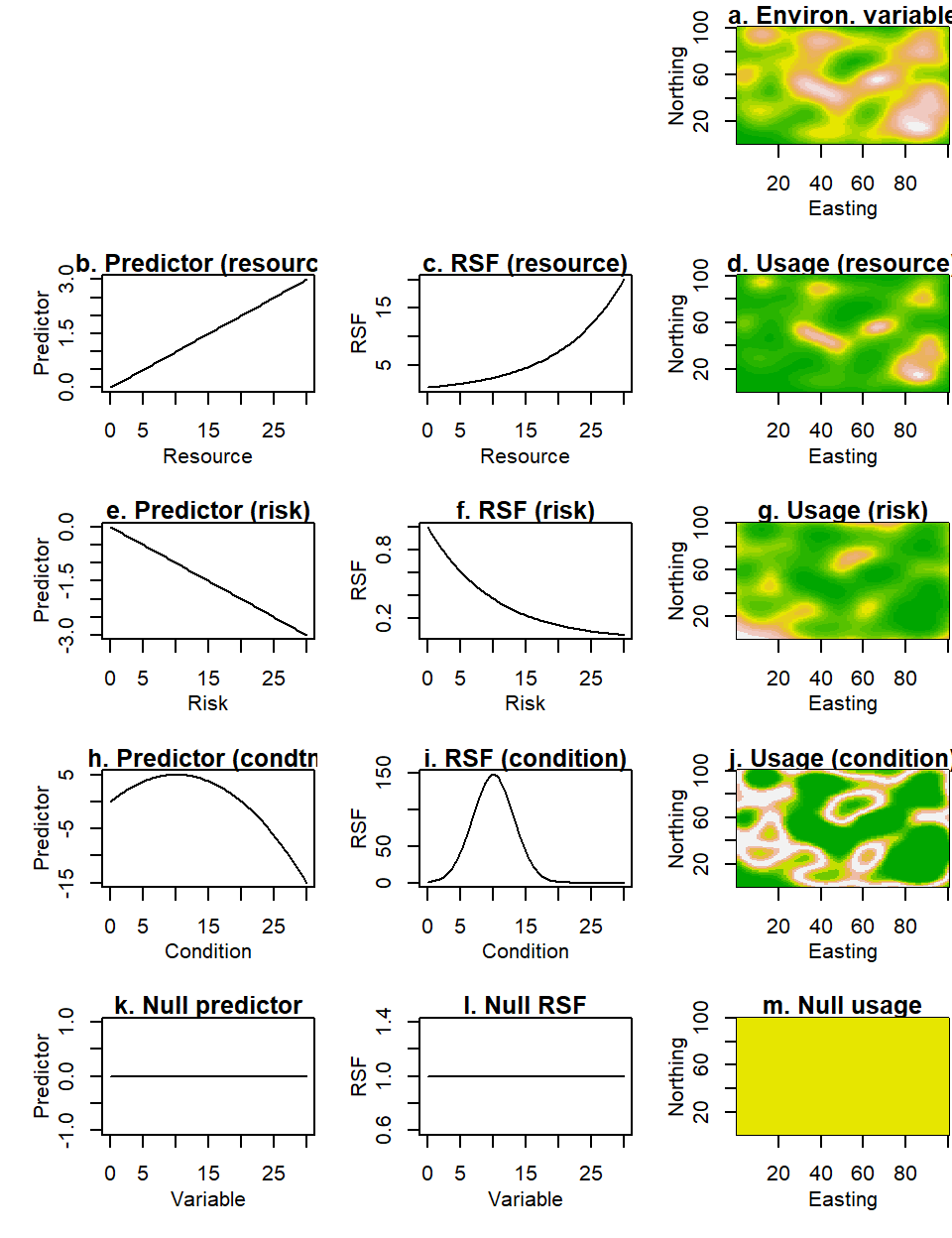
Figure 2.4: Usage in response to different types of variables. Consider the generic layer in (a) which representes the spatial distribution of an environmental variable. In the first and second columns we show the predictor and selection functions assuming that the organism responds to the variable as if it is a resource (b, c), a risk (e, f), a condition (h, i). In the third column (d, g, j) we show the expected distribution of the organism in each of these three scenarios. For completeness, in the bottom row, we show the predictor, selection functions and homogeneous spatial expectation for an organism that is unresponsive to the environmental variable.
2.10 Thinking outside the box: Biological mechanism in process models
Increase in the complexity of the preference function \(h\) can either come from first principles, or the function can acquire added “wiggliness” under the instruction of the data (Wood, 2006). In this section, we look at some immediate extensions that can enhance the biological realism and interpretation of SHA models. We will assume that the form of the preference and selection functions are fixed (as defined in sections 2.7 and 2.8), and we will instead focus on the predictor function. It turns out that, by incorporating simple model features, such as multiple covariates, quadratic terms and interactions, the predictor function can capture a lot of interesting biology.
2.10.1 Single-variable models
Let us start by examining one-dimensional environmental spaces, in the variable \(x\) (Fig. 2.4a shows an example of such a variable in G-space). Our basic classification of habitat characteristics into resources, risks and conditions has an easy mathematical representation (Jason Matthiopoulos et al., 2015). Resources are consistently desirable, so high values of resources should be preferred over low ones. We should therefore expect a positive response to these variables. Risks (assuming they are real and perceived, or just perceived) should have a negative response, indicating avoidance. Therefore, at the scale of the predictor function, we can write
\[\begin{equation} g(x)=\alpha_1 x \tag{2.15} \end{equation}\]
where \(\alpha_1>0\) if \(x\) is a resource and \(\alpha_1<0\) if it is a risk. This assumes the simplest possible form of monotonic relationship between the variable \(x\) and the predictor. Other, more complicated monotonic functions are possible (see e.g. section 2.10.6 on saturating responses), but the biology will need to warrant the use of such additional complexity. However, the proportionality of eq. (2.15) does not mean that such a model’s spatial predictions will be linear. Figs 2.4b & e, show (linear) plots of the predictor for a resource and a risk respectively. The panels right next to them (Figs 2.4c & f) show the exponential version of the same functions (i.e. \(w(x)\), defined, above as the selection function). Finally, the rightmost panels (Figs 2.4d & g) show expected usage in G-space. These maps inherit the nonlinearity and complexity of the underlying environmental variable, but as you might expect, peaks in the resource distribution match the hotspots in expected usage, whereas peaks in risk are coldspots in expected usage.
Response to environmental conditions can be thought of as a combination of the above two scenarios. Consider the example of water availability to an organism. Complete drought is a problem for any plant or animal, so preference should increase together with water availability, initially. After a certain point however, inundation becomes a risk, and preference should decrease with water availability. We therefore need a function that describes such a modal response. The easiest one is a quadratic function
\[\begin{equation} g(x)=\alpha_1 x + \alpha_2 x^2\ \ \ \ \ \ \ \ \alpha_2<0 \tag{2.16} \end{equation}\]
The negative value of \(\alpha_2\) ensures that the graph of \(g(x)\), is a downward-pointing parabola (see Fig. 2.4h). Viewed as an RSF (Fig. 2.4i), this has a rather appealing uni-modal form that anticipates little usage at extreme values of the environmental variable \(x\). When applied to spatial prediction, this model gives us bands of high expected usage (the yellow-white areas in Fig. 2.4j) at intermediate (optimal) values of the condition \(x\). Again, this is the simplest function that can create such a “peaked” response. More complicated functions could be used to ensure, for example, that the curve in Fig. 2.4i is not symmetric, or that it has thicker tails, but an enthusiastic biologist will really need to present a critical modeler with overwhelming evidence to justify such increases in complexity. Even more demanding would be the biological case for a multimodal response to a condition. It is not inconceivable, but seems somewhat less likely (Austin, 1999), that an organism has two optima at different regions of the same variable. It may be argued that such apparent multimodality is the result of responses to more than one variables that have an interactive effect on the organism, so that such phenomena are best modeled in the setting of more than one variables (see section 2.10.3 below).
There is a special case of univariate relationships, indicating absence of preference. An unresponsive relationship \(g(x)=0\) is obtained by setting the coefficients \(\alpha_1\) and \(\alpha_2\) to zero. According to eq. (2.8), this yields a resource-selection function \(w(x)=1\). Placing this into eq. (2.9), we can show that \(h(x)=1\). What does this imply? In environmental space, it means that values of \(x\) are used in proportion to their availability (from eq.(2.4)). In geographical space (see, eq.(2.14)), it means that all points are expected to be used uniformly. These facts are depicted in the bottom three panels of Fig. 2.4.
The above framework captures a wealth of biology with considerable mathematical economy. Using a \(2^{nd}\)-order polynomial \(g(x)=\alpha_1x+\alpha_2x^2\), one of the best-behaved functions in high-school mathematics, we can represent qualitatively different types of variables by selectively switching different \(\alpha\) parameters on and off.
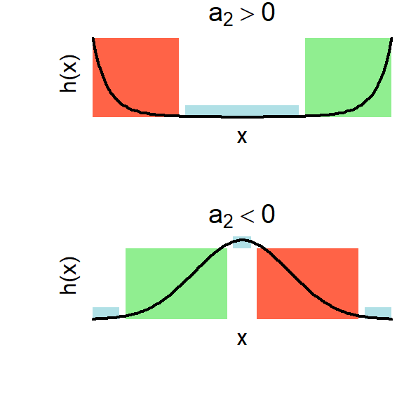
Figure 2.5: Upward and downward pointing parabolas (in the exponential scale corresponding to an RSF) and their biological interpretation over different segments of the environmental variable. The curves behave like resources in the green windows and like risks in the red windows. They appear approximately unresponsive to the environmental variable in the blue regions.
At the same time, this framework also illustrates why it is better to motivate model development from biological first principles rather than mathematical completeness. For example, it is hard to think of a biological reason why an upward-pointing parabola (obtained when \(\alpha_2>0\)) would make sense across the entire range of values of \(x\). However, such a curve might make sense for smaller windows of the full range. In Fig.2.5 we illustrate this point for both upward and downward-pointing parabolas. Different parts of the curve can be used to model different types of responses, if we are prepared to restrict the values of \(x\) (i.e. if we zoom in at selected windows of these plots).
This observation is particularly relevant when data and uncertainty are involved (see Chapter 3). If the window of observed values for \(x\) is sufficiently narrow, and if there is enough fuzziness in the data, then a condition can be misconstrued as a risk and a resource or an irrelevant variable (indicating no response). Indeed, a parabola with a positive value of \(\alpha_2\) may be supported by the data in describing a resource or a condition.
Therefore, it is necessary to use biology to supervise the interpretation of these models. This means that only the first of the following two statements is advisable:
“I know that my species cannot thrive in the absence or in the superabundance of water. I will therefore use a quadratic model to describe its relationship to this variable”
“Within my limited window of data, the species shows a negative/positive response to water. I will therefore conclude that water is a risk/resource for this species”
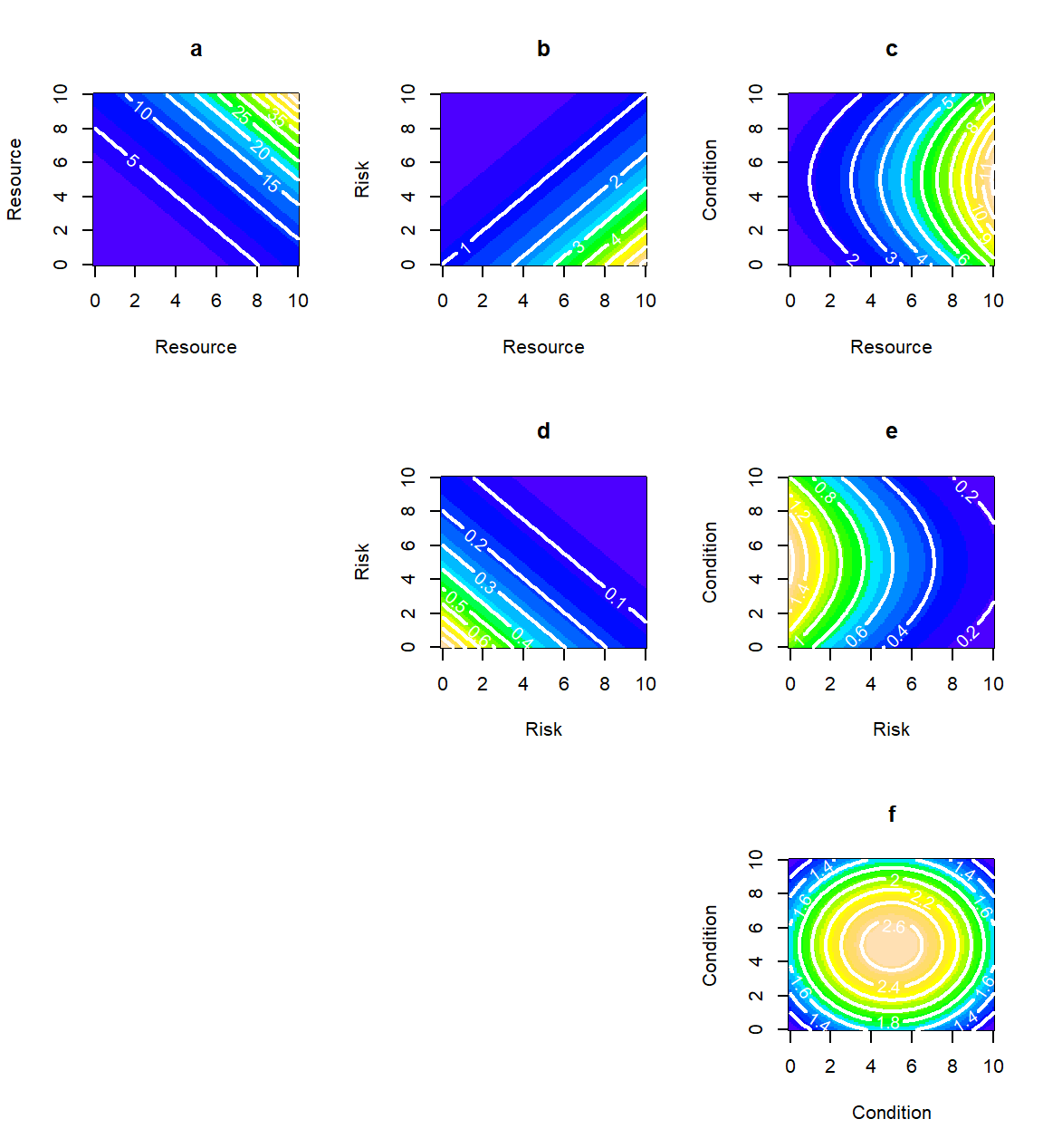
Figure 2.6: Two-variable combinations, generated by pairwise models of resources, risks and conditions. The ramp from cold to warmer colours indicates increasing preference.
2.10.2 Two-variable models: Additive predictors
We can now move on to models with more than one variable. We will generalize on the idea of eq.(2.16), allowing us to look at how combinations of the three basic categories of environmental variables (resources, risks and conditions) behave when they act in tandem. Notionally, to keep track of the extra complexity, we can use a double-subscript \(\alpha_{i,j}\) to indicate that the coefficient belongs to the \(j^{th}\)-order term of the \(i^{th}\) environmental variable.
\[\begin{equation} g(x_1,x_2)=\alpha_{1,1} x_1 + \alpha_{1,2} x_1^2+\alpha_{2,1} x_2 + \alpha_{2,2} x_2^2\ \ \ \ \ \ \ \ \alpha_{1,2},\ \alpha_{2,2}<0 \tag{2.17} \end{equation}\]
By setting the \(\alpha\)’s to positive, negative or zero values, we can create combinations between resources, risks and conditions. These are shown in Fig.(2.6). There are two qualitative points to make here that connect these models with ecological principles.
The shape of fundamental niches: Because SHA models are specified in E-space, there is an understandable tendency to try and interpret them in terms of the ecological niche of a species (Pulliam, 2000; Bahn & Mcgill, 2007; Alexandre H. Hirzel & Le Lay, 2008; Holt, 2009; Warren, 2012, 2013; McInerny & Etienne, 2013). We will examine niche theory in more detail in later chapters, but it is worth broaching the issue early on. The fundamental niche is often described by its Hutchinsonian definition of an “n-dimensional hypervolume”. The image that most textbooks use to visualize it, is akin to our Fig.(2.6f) - areas (or volumes) contained within closed contours in E-space (Blonder, 2018). However, as all the other plates in Fig.(2.6) clearly indicate, functions in E-space need not give rise to closed contours. For instance, there is no reason why the fundamental niche of an organism comprising just resources should be a closed hypervolume, because that would exclude perfectly desirable habitats that just happen to be superabundant in resources (Chase & Leibold, 2003).
There may be a couple of reasons for this misleading imagining of niches in E-space. The botanical origins of these early studies had concentrated on envelopes of temperature, or soil pH that allowed plants to survive. This immediately funnels our thinking into conditions, placing less emphasis on (usually perishable, or depletable) resources and (even less easy to measure) risks. Alternatively, the picture of a closed niche may stem from a confusion between the fundamental niche (what the organism could ideally use) and the realized niche (what it can use within the constraints of its environment). If you refer back to Fig.2.2d you see what appears to be a closed region in E-space (echoing the textbook depictions of Hutchinsonian niches). However, Fig.2.2f more clearly indicates that, once we account for habitat availability, we have a monotonically and diagonally increasing preference, identical in form to our Fig. 2.6a.
Null models for resources and risks: The contours obtained by the combination of linear terms (i.e. resources and risks) are linear (see Figs 2.6a,b and d). This is a useful trait to remember because it gives rise to two ecological null models. The first, is the model of a perfect trade-off between a resource and a risk (Fig.2.6b), which presents increasing contours of preference with a common, constant, slope. Biologically, the slope tells us how many additional units of the resource are needed to balance one additional unit of risk. The second, is the null model of perfectly substitutable resources (Fig.2.6a), a term introduced by Tilman (1982) in his classification of relationships between resources. The linear contours here have a negative slope which represents the “exchange rate” between the two resources (i.e. how much of one resource is needed to replace the loss of a unit of the other resource). We will follow up on this null model in the next section, to relax the assumption of perfect substitutability.
2.10.3 Two-variable models: Multiplicative predictors
In this section we stay with models that contain solely two resources. Tilman (1982) had discussed two further scenarios, for the joint action of resources on organisms, antagonism and complementarity (Fig. 2.7). Two or more resources that can substitute for one another, are called antagonistic if, when taken together, they may partially off-set the effects of each-other. The consumer requires more of the resources when they are taken together than when they are taken separately (Fig. 2.7b). In contrast, complementary (or synergistic) resources augment one another, so that the consumer requires less of them when taken together than when taken separately (Fig. 2.7c). These features can be captured by the general model of two resources with the addition of an interaction term.
\[\begin{equation} g(x_1,x_2)=\alpha_{1} x_1 +\alpha_{2} x_2+\beta_{1,2}x_1x_2 \tag{2.18} \end{equation}\]
Where \(\beta_{1,2}\) is negative for antagonism and positive for complementarity. A rather appealing property of this general model is that the null model of perfect substitutability is nested within it (just set \(\beta_{1,2}=0\)). However, as with earlier models in this chapter, only some parameterizations of eq.(2.18) make biological sense. In particular, the model for antagonism only makes sense for certain values of \(\beta\) which, rather concerningly, depend on the upper limits of values considered for the resource axes6.
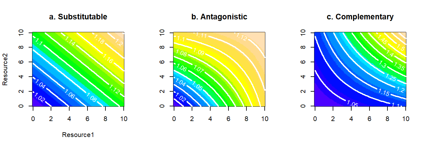
Figure 2.7: Relaxing the assumption of perfect substitutability (shown in a) between two resources, to create antagonism (part b), or complementarity (part c).
2.10.4 Multivariable models
The above principles, readily generalize to more than two habitat variables. For example, the following model
\[\begin{equation} \ g(x_1,x_2,x_3,x_4)=0.1x_1-0.001x_1^2-0.2x_2+0.4x_3+0.002x_3x_4 \end{equation}\]
is rich in biological information and could be decoded as follows: 1. \(x_1\) is a condition; 2. \(x_2\) is a risk, 3. \(x_3\) is a resource; 4. There is a perfect trade-off between \(x_2\) and \(x_3\); 5. For low values of \(x_1\), this condition behaves as a substitutable resource to \(x_3\); 6. High values of \(x_1\) aggravate the effect of the risk \(x_2\) and trade-off against the resource \(x_3\); 7. The organism has no direct response to the variable \(x_4\) (since there is no main term for \(x_4\) the slope of \(g\) in response to \(x_4\) is zero); 8. However, the variable \(x_4\) is able to moderate the response of the organism to variable \(x_3\).
Interpretation of these more complex models becomes much harder as additional terms are introduced, and it becomes increasingly difficult to specify constraints for the parameter values that can keep the behavior of the model within desired biological requirements7.
2.10.5 Functional and multiscale responses in SHA models
All of the extensions of the basic linear model that we have examined until now refer back to a special case of the habitat preference function. In eq.(2.4) we made the explicit assumption that habitat preference is \(h(\mathbf{x})\), i.e. purely a function of local habitat \(\mathbf{x}\). However, the original expression of habitat preference in (2.3) was more flexible than that, allowing for other, e.g. non-local arguments to be used. Two particular topics that have often made their appearance in discussions about SHA models are habitat context and spatial scale. We look at those in turn.
The assumption made by most current studies of habitat selection is that the choices made by organisms (particularly animals) are constant, irrespective of the availability of habitats in their broader neighborhood. However, a mounting body of literature, reviewed in Jason Matthiopoulos, Hebblewhite, Aarts, & Fieberg (2011) and Holbrook et al. (2019), is arguing from the basis of both biological data and theoretical principles that animals modify their choices depending on habitat context. This phenomenon is known as a functional response in habitat selection (Mysterud & Ims, 1998). In the vaguest, most unhelpful terms, we can formalize this as a dependence of habitat preference on the makeup of E-space as a whole (2.8)

Figure 2.8: The response of an organism to any given habitat depends on environmental context, i.e., the availability of all other habitats. Using a restaurant metaphor, a customer who wants to avoid spicy food in an Indian restaurant, may be forced to opt for a relatively mild dish, even if it is not a particular favorite. Given a different environmental context, a strongly preferred dish may become apparent. This phenomenon is known as a functional response in habitat selection.
\[ h(\ )=h(\mathbf{x},f_a)\] However, this does not readily imply a way forward for mathematical modeling. Without throwing the models of the preceding sections to the waste bin, how can we extend our existing mathematical framework of habitat preference functions to account for the effect on space-use of the availability of all habitats in the neighborhood of an animal? Four difficult questions present themselves.
How should we summarize habitat availability? This question cannot be answered easily, but not for lack of answers (far too many possibilities present themselves). The Rolls-Royce approach would use a detailed parametric description of availability \(f_a(\mathbf{x})\) across E-space, such that every little nuance of the variations in habitat availability is captured. A less luxurious approach would focus on each individual habitat variable and describe its frequency distribution \(f_a(x)\) parametrically. A less immediate, but potentially quite detailed method would use a sequence of statistical moments from the distribution of each variable \(E(X),E(X^2),E(X^3),...\). The least powerful approach is to simply use the first of those moments, i.e. the average value of a variable \(\bar{x}=E(X)\). For the rest of this section, let us represent availability by this simplest of summaries. The average value of a variable in the neighborhood of an animal.
How should the availability of a single habitat affect usage? In their review (Holbrook et al., 2019), present four apparently distinct ways in which habitat availability can affect usage. One of those, originally proposed by Boyce & McDonald (1999), suggested that the coefficients of a selection function could be modeled as functions of habitat availability. In statistics, this is known as a varying-coefficient model (Hastie & Tibshirani, 1993). In fact, as we will see in a future chapter, all four of the approaches outlined by Holbrook et al. (2019) can be reduced to a model of varying coefficients. For example, in two of their possible approaches, they debate implicitly the merits of having a direct or interactive effect of availability on the linear predictor of a model. Consider a simple univariate model with predictor
\[\begin{equation} \ g(x)=\alpha_0+\alpha_1 x \tag{2.19} \end{equation}\]
The availability of habitat in the neighborhood of the animal can be introduced by making the coefficients dependent on availability (i.e. \(\alpha_0(\bar{x})\) and \(\alpha_1(\bar{x})\)). We can do this most easily by recasting the \(\alpha\)’s as linear functions of \(\bar{x}\)
\[ \alpha_0(\bar{x})=\beta_{0,0}+\beta_{0,1}\bar{x} \ \ \ \ \ \ \ \ \alpha_1(\bar{x})=\beta_{1,0}+\beta_{1,1}\bar{x} \]
Placing these expressions back into eq. (2.19) gives us both main and multiplicative effects of availability on the linear predictor, in the new \(\beta\) coefficients:
\[ g(x)=\beta_{0,0}+\beta_{0,1}\bar{x}+\beta_{1,0}x+\beta_{1,1}\bar{x}x , \] indicating that we don’t really need to step outside the simple varying-coefficient paradigm to be able to have direct and multiplicative effects of availability on usage. However, from the point of view of interpretation, the existence of a direct term (i.e. \(\beta_{0,1}\bar{x}\)) implies an effect on the intercept (\(\alpha_0\)) of the response, whereas an interactive term (\(\beta_{1,1}\bar{x}x\)) comes from a change in the slope (\(\alpha_1\)) of the predictor.
How should the availability of all habitats on all other habitats be considered simultaneously? If we generalize eq.(2.18) to two habitat variables,
\[ g(x_1,x_2)=\alpha_0+\alpha_1 x_1+\alpha_2x_2 \]
we can also generalize the dependence of model coefficients to more than one expectations, so that \[\alpha_0(\bar{x}_1,\bar{x}_2)=\beta_{0,0}+\beta_{0,1}\bar{x}_1+\beta_{0,2}\bar{x}_2\] \[ \alpha_1(\bar{x}_1,\bar{x}_2)=\beta_{1,0}+\beta_{1,1}\bar{x}_1+\beta_{1,2}\bar{x}_2 \] \[ \alpha_2(\bar{x}_1,\bar{x}_2)=\beta_{2,0}+\beta_{2,1}\bar{x}_1+\beta_{2,2}\bar{x}_2\]
Or, more generally, if we introduce
\[\mathbf{x}= \begin{bmatrix} 1 \\ x_1 \\ \vdots \\ x_K \end{bmatrix}, \ \ \bar{\mathbf{x}}= \begin{bmatrix} 1 \\ \bar{x}_1 \\ \vdots \\ \bar{x}_K \end{bmatrix}, \ \ \beta= \begin{bmatrix} \beta_{0,0} & \ldots & \beta_{0,1}\\ \vdots & \ddots & \vdots \\ \beta_{K,0} & \ldots & \beta_{K,1} \end{bmatrix}, \ \ \alpha=\begin{bmatrix} \alpha_0 \\ \vdots \\ \alpha_K \end{bmatrix}\]
Then the predictor model can be written as
\[\begin{equation} \ g(\mathbf{x}, \bar{\mathbf{x}}) = \alpha^T \mathbf{x} = (\beta \bar{\mathbf{x}})^T\mathbf{x} \end{equation}\]
This is a good starting point for the \(n\)-variable, varying-coefficient model, assuming that both the predictor function and the variations in the coefficients are linear functions.
What is a relevant neighborhood over which to consider availability? As proffered by (Allen & Hoekstra, 1992), “In ecology, looking for the right thing is easier than looking for the right size”. While focusing on such exotica as functional responses, many papers (including several of ours) sweep the question of the scale of availability under the carpet. However, it is important to try and consider, from first principles, what is a relevant scale for calculating habitat availability. For a given temporal scale, presumably the easiest thing is to define a spatial buffer (e.g. a disc), determined by the speed of movement of an animal. However, driving the definition purely by movement capabilities may be misleading. For one, the environment may present obstacles to movement, so that the buffer is not radially symmetric or constant in size. But higher cognitive processes can also interfere. For a large temporal scale, yielding a buffer much larger than an animal’s range of perception, several far-away habitats may be accessible but not perceived. Does this mean they are still available, if they are not explicitly included in the menu from which the individual is making a choice? Alternatively, it can be argued that information is not purely dependent on immediate perception. Memory and communication play a role, effectively extending the range of perception of an animal in non-trivial ways. We will return to these issues of availability in later chapters where we will broaden our examination of functional responses.
Nevertheless, this last question (on scale) prompts the issue of multi-scale selection. Habitat selection happens at multiple spatiotemporal scales (D. H. Johnson, 1980; Mayor, Schneider, Schaefer, & Mahoney, 2009) and statistically, the assumptions of scale, regarding availability can seriously affect our biological inferences (Beyer et al., 2010; Paton S Robert & Matthiopoulos Jason, 2018). So, why have to choose? Why not develop a method that captures multiple scales at the same time? The main challenge here is that every choice made today, necessarily limits the options available for tomorrow. More specifically (DeCesare et al., 2012), there must be a hierarchy of scales so that choices made at finer scales (e.g. minute-to-minute and step-by-step movements between fine-grain habitats) are conditional on choices made at larger scales (e.g. annual or interannual decisions on which broad area to live in).
2.10.6 Saturating responses
One of the main features missing from current formulations of SHA models (but which is quite frequently encountered in nature) is the principle of diminishing returns, the idea that preference does not increase at the same rate with additional increases in resources. The polynomial gold vein we have been mining until now (and that has taken us quite far biologically), becomes exhausted at this point. It is possible to caricature the behavior of a saturating function, using high-order polynomials, within a strictly defined window of habitat values, but that behavior inevitably breaks down under extrapolation (Fig. 2.9).
To capture saturating responses economically and robustly, we need to extend the predictor function to take as arguments more general functions for some of the habitat variables:
\[g(\mathbf{x})=\alpha_0+\sum_{k=1}^{K_1}\alpha_k x_k+\sum_{k=K_1+1}^{K_2} f_k(x_k) \] In theoretical ecology, saturating responses have been captured with a wide range of specific functions, but most often we use fractional and exponential formulae, e.g.
\[f(x)=\frac{\alpha x^c}{\gamma^c+x^c},\ \ \ \ \ f(x)=\alpha(1-exp(-\gamma x^c)),\ \ \ \ (\alpha,\gamma, c >0)\] If you are familiar with consumer-resource models (Murdoch, Briggs, & Nisbet (2003)), you may recognize the first of those functions as the most general (i.e.type III) Holling functional response (Holling (1959)). For example, the curve in Fig 2.9) is derived from the function \(f(x)=10x/(4+x)\).
There is considerable potential for exploring how such curves interplay in predictor functions of multiple variables, particularly given the normalization of the selection function into a preference function.
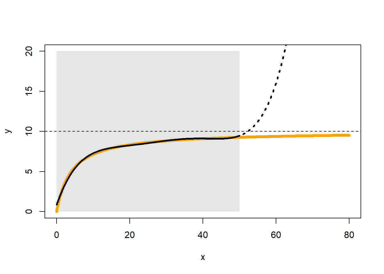
Figure 2.9: Our ability to describe saturating responses with polynomials is limited to the window of approximation (shown in grey) and the approximation is parameter-greedy. The saturating curve shown in orange, approaches an asymptote at the value 10. The approximating polynomial is based on the values of the orange curve within the grey window. It takes a 5th-order polynomial to achieve a convincing approximation (i.e. 6 parameters in total) and the approximation goes awry, immediately after we exit the grey window.
2.11 Concluding remarks
SHA models are formulated in E-space and generate predictions about the expected distribution of a species in G-space. The transition from G-spaces to E-spaces and back again is a central theme to SHA approaches, although it is often done with minimal acknowledgment. Knowing which type of space we are operating in is important, because the transition is not always loss-free. For example, several difficult decisions on how to define habitat availability (an E-space concept) are ultimately questions of geographic accessibility (a G-space concept), but the two are not interchangeable. A model that talks about habitat availability without recognizing the geographic proximity between habitats is, by the same token, a simpler and information-poorer model. The mathematical phrasing of SHA models in E-spaces can be kept quite simple but yet capture a remarkable number of biological phenomena. There are, however, several places where these simple mathematical formulations break down biologically and need to be constrained or made more complex. Traditionally, neither constraints nor complexity have been willingly pursued with SHA models because analysts have always kept foremost in their mind that the of SHA models would need to be derived from field data (and not out of the blue, as we mostly did in this chapter). When fitting models to data, we are bound to look at the resulting responses and interpret them biologically. However, model fitting (the subject of the next chapter) is liable to return parameter values that challenge the interpretive abilities of even the most imaginative biologist. Rather than taking the results of model fitting on-faith (and even worse, generating uncritical predictions from such models), this chapter has hopefully provided the mathematical insights to specify meaningful models, cast meaning to models derived from data, and pursue the development of mathematical constraints and functional complexity to tread the fine line between empiricism and mechanism.
References
Hence, a model that uses longitude and latitude as fixed or random effects is tied to the geographical region in which it was fitted. This may be a good idea when controlling for missing covariates, but in order to predict in other regions the spatial terms must be dropped. Such an approach (i.e. explicitly spatial during the model fitting stage, but non-spatial during the prediction stage) could increase the robustness of predictions by accounting for residual spatial autocorrelation (although it may inadvertently lead to the removal of covariates that are important Hodges & Reich, 2010).↩︎
If you prefer to think in terms of probability, this expression can be written as \(P(Use,Available)=P(Use|Available)P(Available)\). The conditional probability in this expression, represents habitat selection.↩︎
You could think of them as rasters if you prefer to use GIS functionality in R↩︎
To see why that is, consider eq.(2.18). If this ever takes negative values, then we end up with the biologically unrealistic scenario of two resources, acting together as a risk. To avoid that, we need to stipulate that, when \(\beta_{1,2}<0\) (as it must be, to capture antagonistic resources), the net result is always positive. If \(x_{1,max}\) and \(x_{2,max}\) are the upper limits that we are prepared to examine for the two resources, then we require that \[\alpha_{1} x_1 +\alpha_{2} x_2 + \beta_{1,2}x_1x_2 \geq 0.\] This means that \[\beta_{1,2}>-\left( \frac {\alpha_1}{x_{2,max}}+ \frac {\alpha_2}{x_{1,max}}\right).\] In addition, we would like to make sure that our general model is strictly increasing (because it is a response to two resources), so that \[ \frac{\partial g}{\partial{x_1}}, \frac{\partial g}{\partial{x_2}}>0.\] This implies the additional (and more stringent) constraints\[ \beta_{1,2}>max \left({ -\frac{\alpha_1}{x_{1,max}},-\frac{\alpha_2}{x_{2,max}}} \right) .\]↩︎
The role of constrained optimization for fitting SHA models and SDMs is underexplored. As we begin to think about these models more explicitly from the point of view of fitness, it will be sensible to constrain their parameters to plausible ranges (in likelihood approaches) or provide them with more informative priors (in Bayesian approaches).↩︎