Capítulo 7 Como analisar a performance de Modelos de Classificação?
Neste capítulo serão abordadas formas de mensurar a qualidade do ajuste de modelos de classificação, assim como formas de investigar a existência ou não de sobreajuste.
library(tidyverse)
library(rpart)
library(randomForest)
library(xgboost)
base_treino = readRDS(file="arquivos-de-trabalho/base_treino_final.rds")

base_treino = base_treino |>
  mutate(NOTA_RED = ifelse(base_treino$NU_MEDIA_RED>=600,"boa","regular")) |>
  select(-c(CO_ESCOLA_EDUCACENSO,
            NO_ESCOLA_EDUCACENSO,
            NU_MEDIA_CN,NU_MEDIA_CH,
            NU_MEDIA_LP,NU_MEDIA_MT,
            NU_TAXA_PARTICIPACAO,
            NU_PARTICIPANTES,
            NU_MEDIA_RED))

base_treino$NOTA_RED = as.factor(base_treino$NOTA_RED)
7.1 Classificação Binária
Começamos supondo que já temos modelos de classificação. Para o caso deste texto, vamos usar como exemplo a previsão da nota de redação de cada escola entre “boa” e “regular”.
tree_RED = readRDS(file="arquivos-de-trabalho/tree_RED.rds")
rf_RED = readRDS(file = "arquivos-de-trabalho/rf_RED.rds")
xgb_RED = readRDS(file = "arquivos-de-trabalho/xgb_RED.rds")
Suponha que um modelo de classificação \(k\) realizou a previsão \(\hat{y}_i^k\) para a i-ésima observação da variável \(Y\). Como se trata de um modelo de classificação binário, as classes serão 0 ou 1 e a previsão \(\hat{y}_i^k\) é um valor no intervalo \((0,1)\) que indica o quanto provavél a observação está de pertencer à classe de referência, que é a classe 1.
Começamos com a previsão na base de treino. Primeiro para os modelos de árvore e de floresta aleatóra.
prev_treino_tree  = predict(tree_RED,
                              newdata = base_treino,
                              type = "prob")

prev_treino_rf  = predict(rf_RED,
                          newdata = base_treino,
                          type = "prob")
E depois para o modelo XGBoost, que tem uma sintaxe diferente dos anteriores.
M_treino = model.matrix(~., data = base_treino)[,-1]
X_treino = M_treino[,-45]
Y_treino = M_treino[,45]

prev_treino_xgb  = predict(xgb_RED,newdata = X_treino,type = "prob")
Podemos também encontrar previsões para os dados de teste. Nesete caso primeiro devem ser lidos e tratados os dados de teste para então realizar as previsões.
base_teste = readRDS(file="arquivos-de-trabalho/base_teste.rds")
base_teste = base_teste |> select(-c(NU_MEDIA_OBJ,
                                     NU_MEDIA_TOT,
                                     NU_ANO,
                                     NU_TAXA_APROVACAO,
                                     CO_UF_ESCOLA,
                                     CO_MUNICIPIO_ESCOLA,
                                     NO_MUNICIPIO_ESCOLA))
base_teste = base_teste  |>
  mutate(NU_TAXA_REPROVACAO = replace_na(NU_TAXA_REPROVACAO, mean(base_treino$NU_TAXA_REPROVACAO, na.rm = TRUE)),
         NU_TAXA_ABANDONO = replace_na(NU_TAXA_ABANDONO, mean(base_treino$NU_TAXA_ABANDONO, na.rm = TRUE)),
         PC_FORMACAO_DOCENTE = replace_na(PC_FORMACAO_DOCENTE, mean(base_treino$PC_FORMACAO_DOCENTE, na.rm = TRUE))
  )

base_teste = base_teste |>
  mutate(NOTA_RED = ifelse(base_teste$NU_MEDIA_RED>=600,"boa","regular")) |>
  select(-c(CO_ESCOLA_EDUCACENSO,
            NO_ESCOLA_EDUCACENSO,
            NU_MEDIA_CN,NU_MEDIA_CH,
            NU_MEDIA_LP,NU_MEDIA_MT,
            NU_TAXA_PARTICIPACAO,
            NU_PARTICIPANTES,
            NU_MEDIA_RED))
Previsão na base de teste.
prev_teste_tree  = predict(tree_RED,
                           newdata = base_teste,
                           type = "prob")

prev_teste_rf  = predict(rf_RED,newdata = base_teste,type = "prob")


M_teste = model.matrix(~., data = base_teste)[,-1]
X_teste = M_teste[,-45]
Y_teste = M_teste[,45]

prev_teste_xgb  = predict(xgb_RED,newdata = X_teste,type = "prob")
7.1.1 Medidas de qualidade do ajuste
Existem algumas possíveis medidas de desempenho para modelos de classificação. As duas mais usuais são a Entropia Cruzada e a Área embaixo da Curva ROC.
7.1.1.1 Entropia Cruzada
Uma vez conhecidas as previsões para a variável resposta, considerando que essas previsões serão uma probbailidade da observação pertencer a classe de referência, é possível calcular a EC (entropia cruzada) e usar essa medida como comparação de qualidade do ajuste.
\[ EC = - \dfrac{1}{N} \sum_{i=1}^N \left( y_i\ln(\hat{y}_i) + (1-y_i)\ln(1-\hat{y}_i) \right) \]
Veja que quando \(\hat{y}_i\) está próximo da classe real a parcela \(i\) do somatório é bem pequena e quando \(\hat{y}_i\) está próxima da classificação errada, a parcela \(i\) do somatório é bem grande. Quanto menor a EC, melhor o ajuste do modelo.
EC = function(real,previsao){
  n = length(real)
  ec = -sum(ifelse(real_treino==1,log(previsao),log(1-previsao)))/n
  return(ec)
}
Veja que a conta acima pode ser feita considerando tanto a base de treino quanto a base de teste. Em geral vamos medir a EC para as duas bases.
Valores da EC para a base de treino.
real_treino = ifelse(base_treino$NOTA_RED == "regular",1,0)

EC_treino_tree = EC(real_treino,prev_treino_tree [,2])

EC_treino_rf = EC(real_treino,prev_treino_rf [,2])

EC_treino_xgb = EC(real_treino,prev_treino_xgb )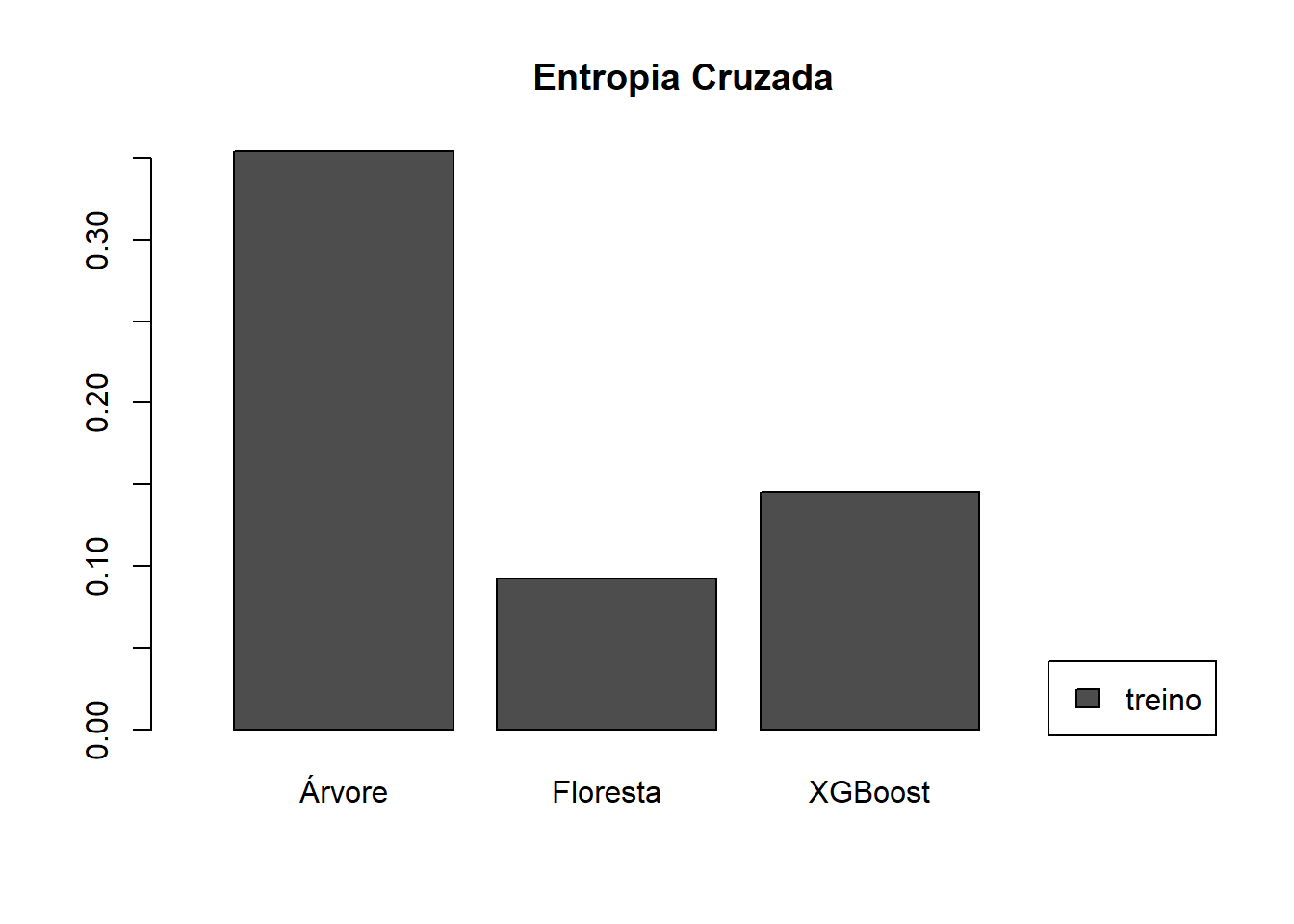
Valores da EC para a base de teste.
#referencia = classe regular
real_teste = ifelse(base_teste$NOTA_RED == "regular",1,0)

EC_teste_tree = EC(real_teste,prev_teste_tree [,2])

EC_teste_rf = EC(real_teste,prev_teste_rf [,2])

EC_teste_xgb = EC(real_teste,prev_teste_xgb )
## Árvore Floresta XGBoost
## EC no treino 0.3541748 0.09241238 0.1453029
## EC no teste 2.9102760 Inf 4.6709746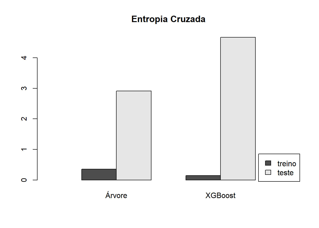
7.1.1.2 Curva ROC
Mas qual valor escolher para \(q\)? A escolha do valor de corte \(q\) pode ser feita a partir da curva ROC. A curva ROC é uma curva parametrizada pelo valor \(q\) definida por:
\[ ROC(q) = (1-Especificidade(q)\ , \ Sensibilidade(q)) \ , \quad q \in (0,1) \]
A figura a seguir mostra como em geral é a curva ROC.
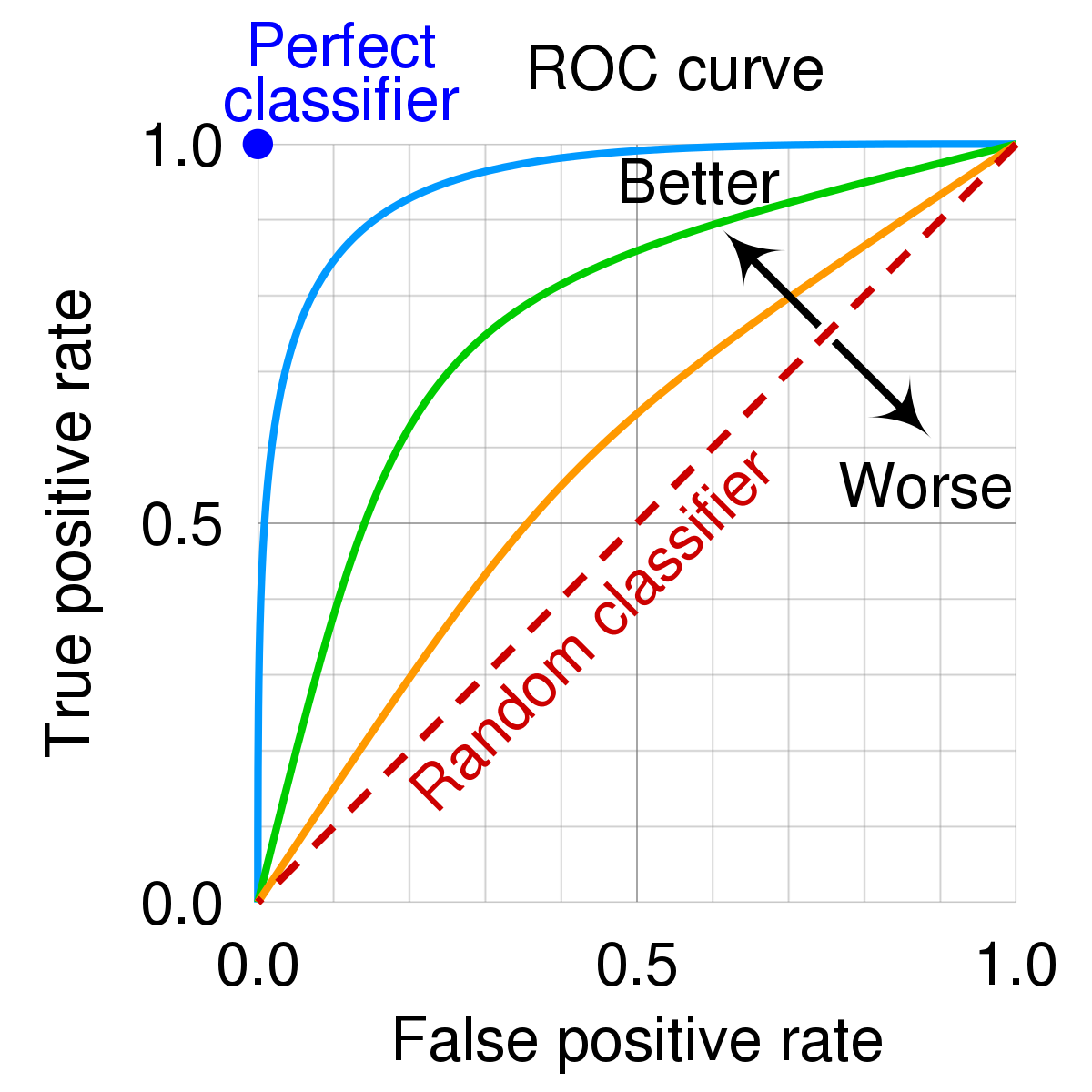
Figura 7.1: Curva ROC
Vamos escolher o valor de \(q\) que gerou o ponto mais acima e à esquerda. O valor da área embaixo da curva ROC (AUC) também é uma medida de qualidade do ajuste bastante usada.
library(pROC)

roc_tree_treino = roc(response = real_treino,
               predictor = prev_treino_tree[,2])
plot.roc(roc_tree_treino,print.auc = TRUE)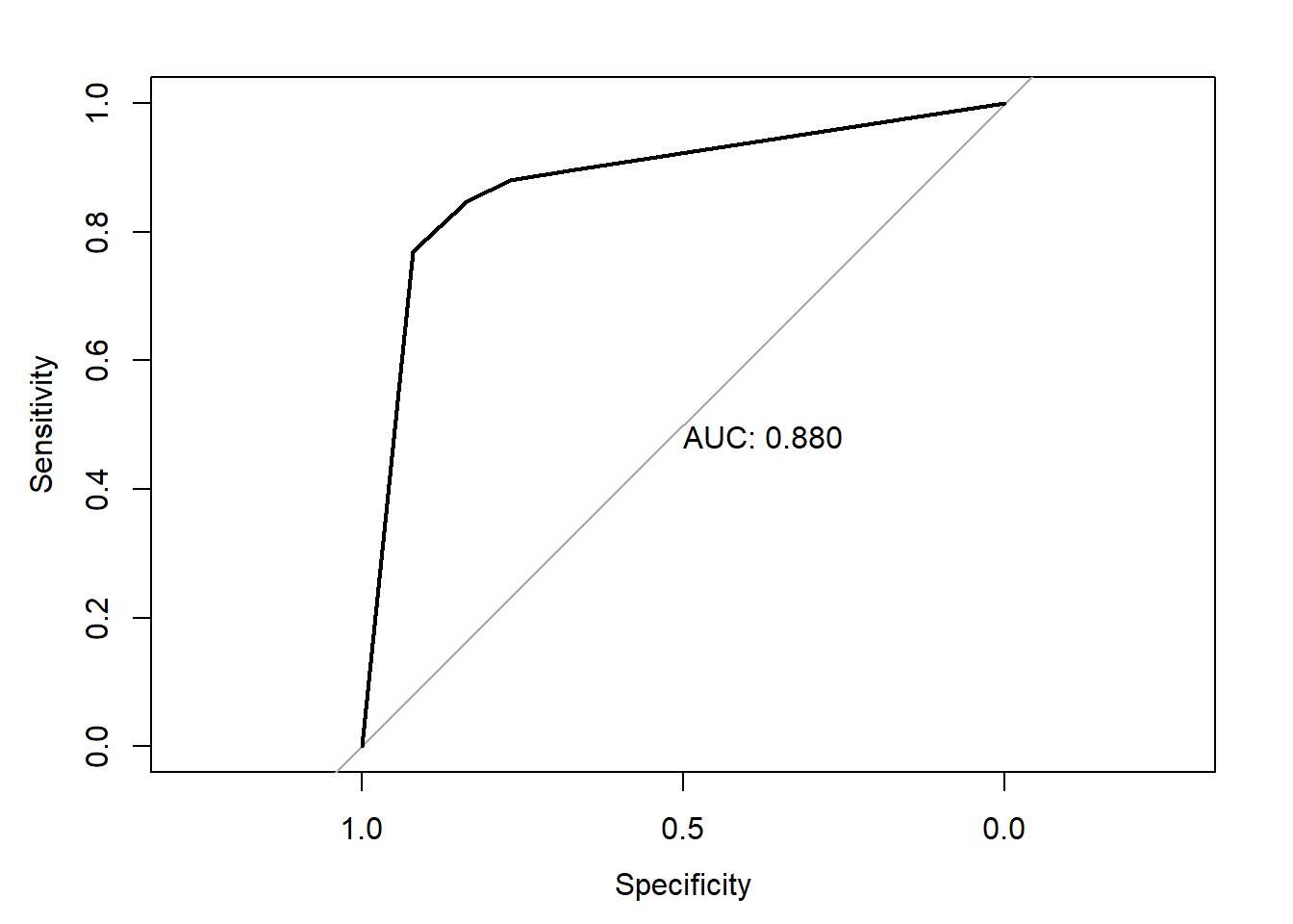
roc_rf_treino = roc(response = real_treino,
               predictor = prev_treino_rf[,2])
plot.roc(roc_rf_treino,print.auc = TRUE)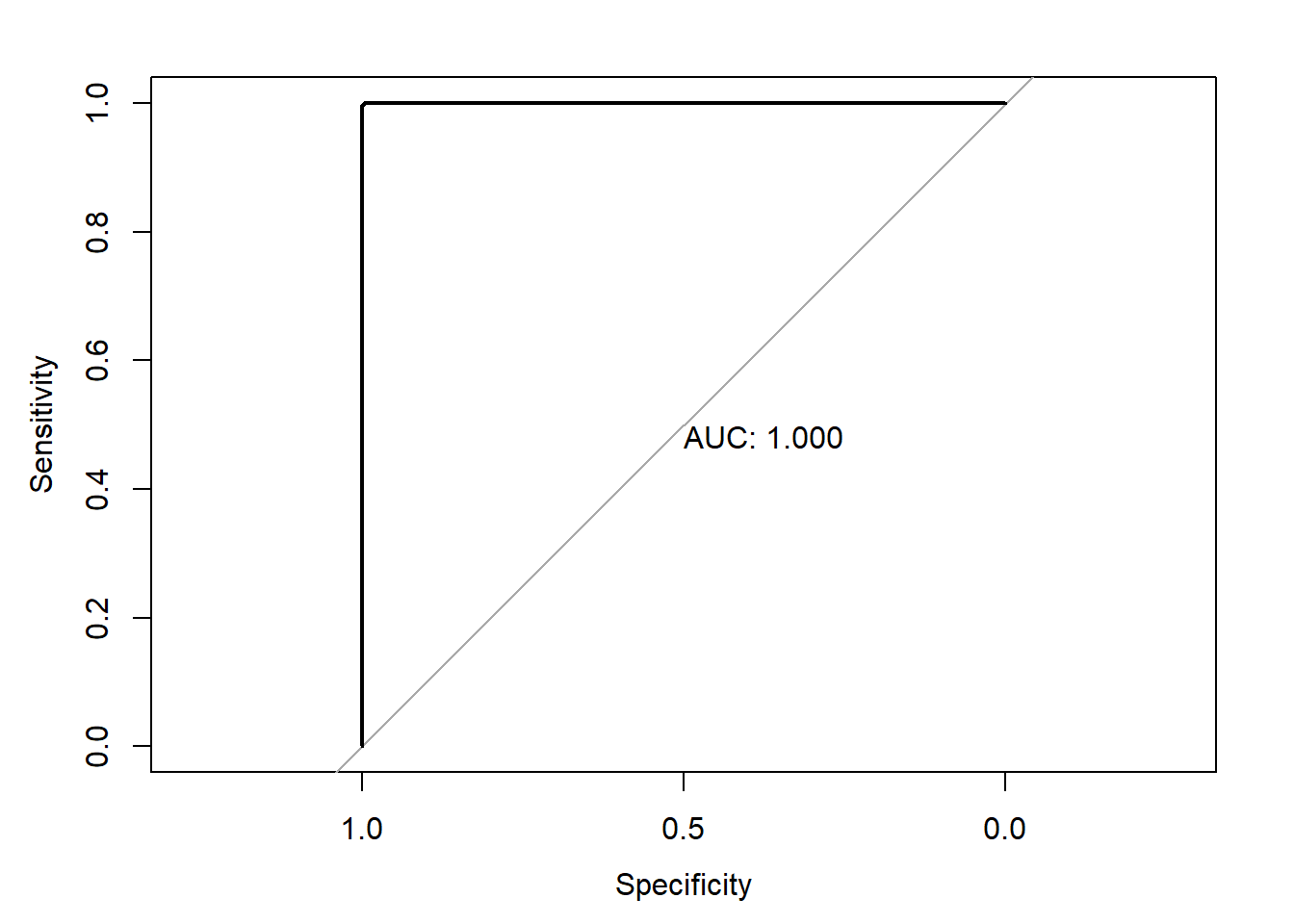
## Area under the curve: 1roc_xgb_treino = roc(response = real_treino,
predictor = prev_treino_xgb )
plot.roc(roc_xgb_treino,print.auc = TRUE)
## Area under the curve: 0.9906A medida de AUC também pode ser encntrada para a base de teste.
roc_tree_teste = roc(response = real_teste,
                      predictor = prev_teste_tree [,2])
plot.roc(roc_tree_teste,print.auc = TRUE)
## Area under the curve: 0.8746roc_rf_teste = roc(response = real_teste,
predictor = prev_teste_rf [,2])
plot.roc(roc_rf_teste,print.auc = TRUE)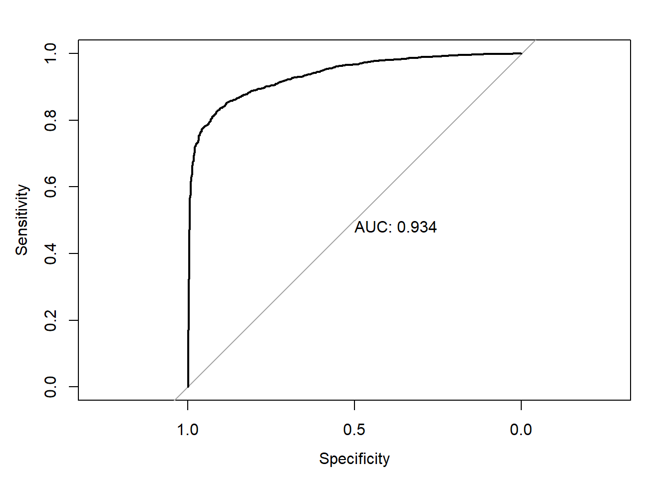
## Area under the curve: 0.9342roc_xgb_teste = roc(response = real_teste,
predictor = prev_teste_xgb )
plot.roc(roc_xgb_teste,print.auc = TRUE)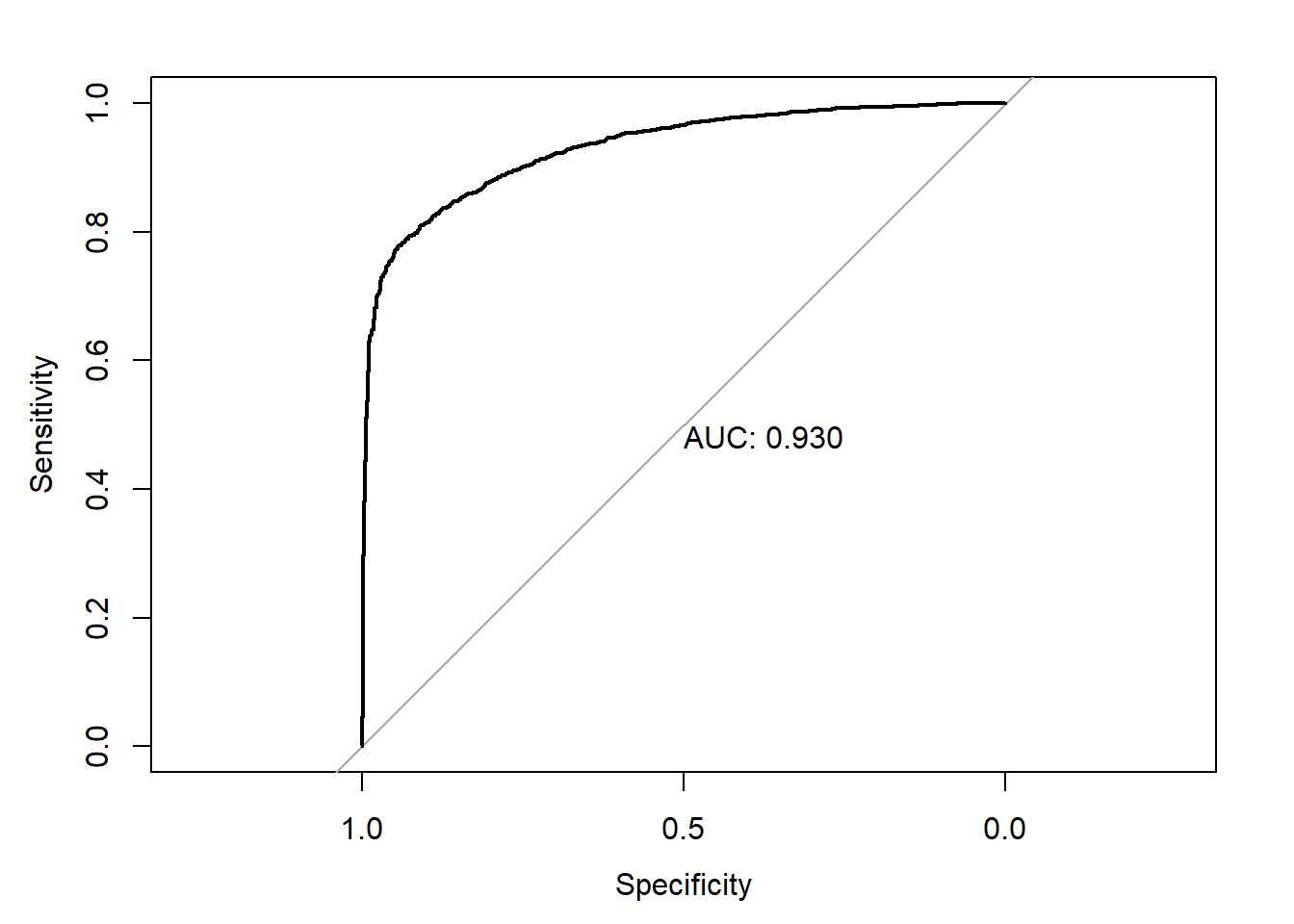
## Area under the curve: 0.93df2 = data.frame(arvore = roc_tree_teste$auc,
floresta = roc_tree_teste$auc,
xgboost = roc_tree_teste$auc)
rownames(df2) = c("AUC no teste")
colnames(df2) = c("Árvore","Floresta","XGBoost")
rbind(df,df2)## Árvore Floresta XGBoost
## AUC no treino 0.8797110 0.9999862 0.9906083
## AUC no teste 0.8745771 0.8745771 0.8745771barplot(as.matrix(rbind(df,df2)),
beside = TRUE,
ylim=c(0,1),
xlim = c(0,11),
legend.text = c("treino","teste"),
names.arg = c("Árvore","Floresta","XGBoost"),
args.legend = list(x="bottomright"),
main = "Entropia Cruzada")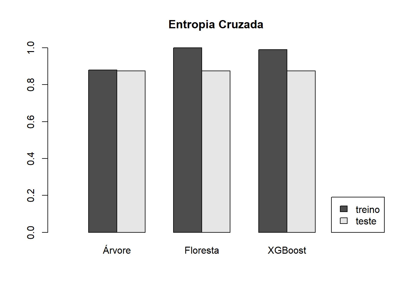
7.1.2 Validação Cruzada para Classificação
7.1.2.1 Árvres de Classificação
param = list(minsplit = c(20,10,50),
             cp = c(0.01, 0.005, 0.02),
             maxdepth = c(30,20,10))

param_combination_tree = expand.grid(param, stringsAsFactors = FALSE)
AUC_treino_tree = matrix(NA,nrow = nrow(param_combination_tree),ncol = K)
AUC_valida_tree = matrix(NA,nrow = nrow(param_combination_tree),ncol = K)
for(i in 1:nrow(param_combination_tree)){
print(i)
for(f in 1:K){
print(f)
valida = base_treino |> dplyr::slice(indices_folds[[f]])
treino = base_treino |> dplyr::slice(-indices_folds[[f]])
tree <- rpart(NOTA_RED ~ .,
data = treino,
method = "class",
control = rpart.control(minsplit = param_combination_tree$minsplit[i],
cp = param_combination_tree$cp[i],
maxdepth = param_combination_tree$maxdepth[i]))
prev_treino = predict(tree,newdata = treino,type="prob")
prev_valida = predict(tree,newdata = valida,type="prob")
classe_treino = treino$NOTA_RED
classe_valida = valida$NOTA_RED
AUC_treino_tree[i,f] = (roc(response = classe_treino, predictor = prev_treino[,2]))$auc
AUC_valida_tree[i,f] = (roc(response = classe_valida, predictor = prev_valida[,2]))$auc
}
}result_treino_tree =
apply(AUC_treino_tree, MARGIN = 1, summary)
result_valida_tree =
apply(AUC_valida_tree, MARGIN = 1, summary)mat = matrix(c(
result_treino_tree["Mean",],
result_valida_tree["Mean",]),
byrow = TRUE,
nrow=2)
barplot(mat,
names.arg = 1:nrow(param_combination_tree),
beside = T,
ylim = c(0,1),
xlim = c(0,90),
main="AUC para Validação Cruzada do Árvore",
legend.text = c("treino","valida"),
args.legend = list(x="bottomright"))
abline(h=min(mat),lty=2,col="lightgray")
7.1.2.2 Floresta Aleatória
param = list(mtry = c(2,3,4),
             ntree = c(100,500))

param_combination_rf = expand.grid(param, stringsAsFactors = FALSE)
AUC_treino_rf = matrix(NA,nrow = nrow(param_combination_rf),ncol = K)
AUC_valida_rf = matrix(NA,nrow = nrow(param_combination_rf),ncol = K)
for(i in 1:nrow(param_combination_rf)){
print(i)
for(f in 1:K){
print(f)
valida = base_treino |> dplyr::slice(indices_folds[[f]])
treino = base_treino |> dplyr::slice(-indices_folds[[f]])
rf <- randomForest(NOTA_RED ~ .,
data = treino,
mtry = param_combination_rf$mtry[i],
ntree = param_combination_rf$ntree[i])
prev_treino = predict(rf,newdata = treino,type="prob")
prev_valida = predict(rf,newdata = valida,type="prob")
classe_treino = treino$NOTA_RED
classe_valida = valida$NOTA_RED
AUC_treino_rf[i,f] = (roc(response = classe_treino, predictor = prev_treino[,2]))$auc
AUC_valida_rf[i,f] = (roc(response = classe_valida, predictor = prev_valida[,2]))$auc
}
}result_treino_rf =
apply(AUC_treino_rf, MARGIN = 1, summary)
result_valida_rf =
apply(AUC_valida_rf, MARGIN = 1, summary)
7.1.2.3 XGBoost
param = list(eta = c(0.1,0.05,0.15),
             subsample = c(0.5, 0.4, 0.6),
             nrounds = c(100, 200))

param_combination_xgb = expand.grid(param, stringsAsFactors = FALSE)
AUC_treino_xgb = matrix(NA,nrow = nrow(param_combination_xgb),ncol = K)
AUC_valida_xgb = matrix(NA,nrow = nrow(param_combination_xgb),ncol = K)
for(i in 1:nrow(param_combination_xgb)){
print(i)
for(f in 1:K){
print(f)
valida = base_treino |> dplyr::slice(indices_folds[[f]])
treino = base_treino |> dplyr::slice(-indices_folds[[f]])
M_treino = model.matrix(~., data = treino)[,-1]
X_treino = M_treino[,-45]
Y_treino = M_treino[,45]
M_valida = model.matrix(~., data = valida)[,-1]
X_valida = M_valida[,-45]
Y_valida = M_valida[,45]
xgb <- xgboost(data = X_treino,
label = Y_treino,
objective = "binary:logistic",
nrounds = param_combination_xgb$nrounds[i],
subsample = param_combination_xgb$subsample[i],
eta = param_combination_xgb$eta[i])
prev_treino = predict(xgb,newdata = X_treino,type="prob")
prev_valida = predict(xgb,newdata = X_valida,type="prob")
classe_treino = treino$NOTA_RED
classe_valida = valida$NOTA_RED
AUC_treino_xgb[i,f] = (roc(response = classe_treino, predictor = prev_treino))$auc
AUC_valida_xgb[i,f] = (roc(response = classe_valida, predictor = prev_valida))$auc
}
}AUC_treino_xgb = readRDS(file="AUC_treino_xgb.rds")
AUC_valida_xgb = readRDS(file="AUC_valida_xgb.rds")result_treino_xgb =
apply(AUC_treino_xgb, MARGIN = 1, summary)
result_valida_xgb =
apply(AUC_valida_xgb, MARGIN = 1, summary)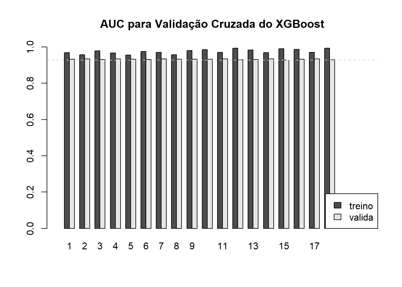
7.1.3 Medidas de qualidade da classificação
Mas como medir a capacidade de classificação?
7.1.3.1 Matriz de Confusão
Os modelos de classificação retornam como previsão para a \(i\)-ésima observação um valor \(\hat{y}_i^k \in (0,1)\). Mas o objetivo final é prever a classe da observação \(i\).
Uma vez escolhido o modelo de classificação que melhor se ajusta aos dados, podemos realizar agora a previsão da classe para a observação \(i\). Suponha o seguinte critério para a escolha da classe prevista:
\[ \hat{c}_i = \left\{ \begin{array}{ll} 0 & \hbox{, se } \hat{y}_i < q\\ 1 & \hbox{, se } \hat{y}_i \ge q\\ \end{array} \right. \]
O valor de \(q\) pode ser determinado a partir da curva ROC para os dados de treino.
Para entender melhor a capacidade de previsão do modelo de classificação queremos encontrar as medidas de Acurácia, Precisão, Sensibilidade, entre outras. Estas medidas serão definidas a partir da matriz de confusão, que é formada pela contagem de classes reais e classes previstas.
| Real 0 | Real 1 | |
| Prev 0 | VN | FN |
| Prev 1 | FP | VP |
VN = verdadeiro negativo = número de observações iguais a 0 que foram previstas como 0.
FN = falso negativo = número de observações iguais a 1 que foram previstas como 0.
FP = falso positivo = número de observações iguais a 0 que foram previstas como 1.
VP = verdadeiro positivo = número de observações iguais a 1 que foram previstas como 1.
Quanto maior o número de observações na diagonal principal da matriz de confusão melhor. A partir desta tabela podemos calcular algumas medidas de desempenho para os modelos de classificação.
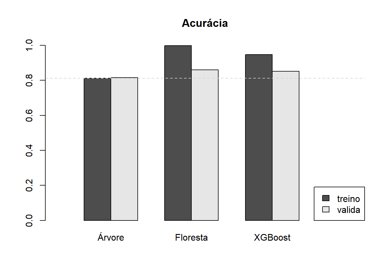
7.1.3.2 Acurácia
A acurácia é a taxa de acerto do classificador. Ela é a proporção de predições corretas dentre todas as predições.
\[ Acurácia = \dfrac{V P + V N}{V P + V N + FP + FN} \]
7.1.3.3 Sensibilidade (ou Recall)
A sensibilidade é a taxa de acerto dos casos positivos. Ela é a proporção de casos positivos que foram corretamente classificados como positivos.
\[ Sensibilidade = \dfrac{VP}{VP + FN} \]
7.1.3.4 Especificidade
A especificidade é a taxa de acerto dos casos negativos. Ela é a proporção dos casos negativos que foram corretamente classificados como negativos.
\[ Especificidade = \dfrac{VN}{V N + FP} \]
7.1.3.5 Precisão
A precisão é a taxa de acerto dentras previsões positivas. Ela é a proporção dos acertos entre os casos classificados como positivos.
\[ Precisão = \dfrac{VP}{V P + FP} \]
7.1.3.6 F1-Score
É uma combinação da Precisão e do Recall que na prática é a média harmônica entre a Precisão e o Recall.
\[ F1-score = 2 \dfrac{Precisão \times Recall}{Precisão + Recall} \]
q_tree = coords(roc_tree_treino, "best", ret = "threshold")[1,1]

prev_class_treino_tree =
  ifelse(prev_treino_tree[,2] > q_tree,"regular","boa")

tabela = table(prev=prev_class_treino_tree,
               real_treino=classe_treino)
CM_treino_tree = confusionMatrix(tabela)
CM_treino_tree
## Confusion Matrix and Statistics
##
## real_treino
## prev boa regular
## boa 3056 1936
## regular 266 6442
##
## Accuracy : 0.8118
## 95% CI : (0.8046, 0.8188)
## No Information Rate : 0.7161
## P-Value [Acc > NIR] : < 2.2e-16
##
## Kappa : 0.5981
##
## Mcnemar's Test P-Value : < 2.2e-16
##
## Sensitivity : 0.9199
## Specificity : 0.7689
## Pos Pred Value : 0.6122
## Neg Pred Value : 0.9603
## Prevalence : 0.2839
## Detection Rate : 0.2612
## Detection Prevalence : 0.4267
## Balanced Accuracy : 0.8444
##
## 'Positive' Class : boa
## q_rf = coords(roc_rf_treino, "best", ret = "threshold")[1,1]
prev_class_treino_rf =
ifelse(prev_treino_rf[,2] > q_rf,"regular","boa")
tabela = table(prev=prev_class_treino_rf,
real_treino=classe_treino)
CM_treino_rf = confusionMatrix(tabela)
CM_treino_rf## Confusion Matrix and Statistics
##
## real_treino
## prev boa regular
## boa 3320 24
## regular 2 8354
##
## Accuracy : 0.9978
## 95% CI : (0.9967, 0.9985)
## No Information Rate : 0.7161
## P-Value [Acc > NIR] : < 2.2e-16
##
## Kappa : 0.9945
##
## Mcnemar's Test P-Value : 3.814e-05
##
## Sensitivity : 0.9994
## Specificity : 0.9971
## Pos Pred Value : 0.9928
## Neg Pred Value : 0.9998
## Prevalence : 0.2839
## Detection Rate : 0.2838
## Detection Prevalence : 0.2858
## Balanced Accuracy : 0.9983
##
## 'Positive' Class : boa
## q_xgb = coords(roc_xgb_treino, "best", ret = "threshold")[1,1]
prev_class_treino_xgb =
ifelse(prev_treino_xgb > q_xgb,"regular","boa")
tabela = table(prev=prev_class_treino_xgb,
real_treino=classe_treino)
CM_treino_xgb = confusionMatrix(tabela)
CM_treino_xgb## Confusion Matrix and Statistics
##
## real_treino
## prev boa regular
## boa 3173 471
## regular 149 7907
##
## Accuracy : 0.947
## 95% CI : (0.9428, 0.951)
## No Information Rate : 0.7161
## P-Value [Acc > NIR] : < 2.2e-16
##
## Kappa : 0.8734
##
## Mcnemar's Test P-Value : < 2.2e-16
##
## Sensitivity : 0.9551
## Specificity : 0.9438
## Pos Pred Value : 0.8707
## Neg Pred Value : 0.9815
## Prevalence : 0.2839
## Detection Rate : 0.2712
## Detection Prevalence : 0.3115
## Balanced Accuracy : 0.9495
##
## 'Positive' Class : boa
## Os resultados podem ser encontrados também para os dados de teste.
prev_class_teste_tree =
  ifelse(prev_teste_tree[,2] > q_tree,"regular","boa")

tabela = table(prev=prev_class_teste_tree,
               real_treino=classe_teste)
CM_teste_tree = confusionMatrix(tabela)
CM_teste_tree
## Confusion Matrix and Statistics
##
## real_treino
## prev boa regular
## boa 1029 632
## regular 87 2150
##
## Accuracy : 0.8155
## 95% CI : (0.803, 0.8276)
## No Information Rate : 0.7137
## P-Value [Acc > NIR] : < 2.2e-16
##
## Kappa : 0.6062
##
## Mcnemar's Test P-Value : < 2.2e-16
##
## Sensitivity : 0.9220
## Specificity : 0.7728
## Pos Pred Value : 0.6195
## Neg Pred Value : 0.9611
## Prevalence : 0.2863
## Detection Rate : 0.2640
## Detection Prevalence : 0.4261
## Balanced Accuracy : 0.8474
##
## 'Positive' Class : boa
## prev_class_teste_rf =
ifelse(prev_teste_rf[,2] > q_rf,"regular","boa")
tabela = table(prev=prev_class_teste_rf,
real_treino=classe_teste)
CM_teste_rf = confusionMatrix(tabela)
CM_teste_rf## Confusion Matrix and Statistics
##
## real_treino
## prev boa regular
## boa 844 274
## regular 272 2508
##
## Accuracy : 0.8599
## 95% CI : (0.8486, 0.8707)
## No Information Rate : 0.7137
## P-Value [Acc > NIR] : <2e-16
##
## Kappa : 0.6574
##
## Mcnemar's Test P-Value : 0.9659
##
## Sensitivity : 0.7563
## Specificity : 0.9015
## Pos Pred Value : 0.7549
## Neg Pred Value : 0.9022
## Prevalence : 0.2863
## Detection Rate : 0.2165
## Detection Prevalence : 0.2868
## Balanced Accuracy : 0.8289
##
## 'Positive' Class : boa
## prev_class_teste_xgb =
ifelse(prev_teste_xgb > q_xgb,"regular","boa")
tabela = table(prev=prev_class_teste_xgb,
real_treino=classe_teste)
CM_teste_xgb = confusionMatrix(tabela)
CM_teste_xgb## Confusion Matrix and Statistics
##
## real_treino
## prev boa regular
## boa 909 369
## regular 207 2413
##
## Accuracy : 0.8522
## 95% CI : (0.8407, 0.8632)
## No Information Rate : 0.7137
## P-Value [Acc > NIR] : < 2.2e-16
##
## Kappa : 0.6535
##
## Mcnemar's Test P-Value : 1.969e-11
##
## Sensitivity : 0.8145
## Specificity : 0.8674
## Pos Pred Value : 0.7113
## Neg Pred Value : 0.9210
## Prevalence : 0.2863
## Detection Rate : 0.2332
## Detection Prevalence : 0.3279
## Balanced Accuracy : 0.8409
##
## 'Positive' Class : boa
## Usando, por exemplo, a acurácia como medida de comparação, temos o seguinte resultado.
7.2 Classificação Multiclasses
Suponha um problema de classificação que, em vez de cada instância (observação) pertencer a uma de duas possíveis classes, ela pertence a uma entre \(k\) possíveis classes.
base_treino = readRDS(file="arquivos-de-trabalho/base_treino_final.rds")


base_treino = base_treino |>
  mutate(NOTA_RED =
           ifelse(
             base_treino$NU_MEDIA_RED>600,"boa",
             ifelse(base_treino$NU_MEDIA_RED<500,"ruim",
                    "regular"))) |>
  select(-c(CO_ESCOLA_EDUCACENSO,
            NO_ESCOLA_EDUCACENSO,
            NU_MEDIA_CN,NU_MEDIA_CH,
            NU_MEDIA_LP,NU_MEDIA_MT,
            NU_TAXA_PARTICIPACAO,
            NU_PARTICIPANTES,
            NU_MEDIA_RED))
base_treino$NOTA_RED = as.factor(base_treino$NOTA_RED)
7.2.1 Medidas de qualidade do ajuste
tree_RED = readRDS(file="arquivos-de-trabalho/tree_RED_3.rds")
rf_RED = readRDS(file = "arquivos-de-trabalho/rf_RED_3.rds")
xgb_RED = readRDS(file = "arquivos-de-trabalho/xgb_RED_3.rds")
7.2.1.1 Previsão na base de treino
prev_treino_tree  = predict(tree_RED,
                            newdata = base_treino,
                            type = "prob")

prev_treino_rf  = predict(rf_RED,
                          newdata = base_treino,
                          type = "prob")


M_treino = model.matrix(~., data = base_treino)[,-1]
X_treino = M_treino[,-c(45,46)]


prev_treino_xgb  = predict(xgb_RED,
                           newdata = X_treino)
prev_treino_xgb =
  matrix(predict(xgb_RED, newdata = X_treino),
         byrow = TRUE,
         ncol=3,
         dimnames = list(NULL,c("boa","regular","ruim"))
  )
7.2.1.2 Entropia Cruzada
Para o caso do problema com mais de duas classes a expressão da entropia cruzada precisa ser generalizada.
\[ EC = - \dfrac{1}{N} \sum_{i=1}^N \sum_{k=1}^K y_{k,i}\ln(\hat{y}_{k,i}) \] sendo, \(N\) o número de instâncias (observações), \(K\) o número de classes, \(y_{k,i}\) a variável indicadora da classe \(k\), isto é, \(y_{k,i} = 1\) se a isntância \(i\) pertence a classe \(k\) e 0 caso contrário, e \(\hat{y}_{k,i}\) o valor de saída para a classe \(k\).
7.2.2 Medidas de qualidade da classificação
7.2.2.1 Previsão da classe na base de treino
classe_treino = base_treino$NOTA_RED

indice_classe = apply(prev_treino_tree,MARGIN = 1,which.max)
prev_class_treino_tree =
  ifelse(indice_classe == 1,"boa",ifelse(indice_classe == 2,"regular","ruim"))

tabela = table(prev=prev_class_treino_tree,
               real_treino=classe_treino)
CM_treino_tree = confusionMatrix(tabela)
CM_treino_tree
## Confusion Matrix and Statistics
##
## real_treino
## prev boa regular ruim
## boa 2745 1271 36
## regular 492 4159 1267
## ruim 41 696 993
##
## Overall Statistics
##
## Accuracy : 0.675
## 95% CI : (0.6664, 0.6834)
## No Information Rate : 0.5236
## P-Value [Acc > NIR] : < 2.2e-16
##
## Kappa : 0.4664
##
## Mcnemar's Test P-Value : < 2.2e-16
##
## Statistics by Class:
##
## Class: boa Class: regular Class: ruim
## Sensitivity 0.8374 0.6789 0.43249
## Specificity 0.8448 0.6844 0.92163
## Pos Pred Value 0.6774 0.7028 0.57399
## Neg Pred Value 0.9303 0.6598 0.86931
## Prevalence 0.2802 0.5236 0.19624
## Detection Rate 0.2346 0.3555 0.08487
## Detection Prevalence 0.3463 0.5058 0.14786
## Balanced Accuracy 0.8411 0.6817 0.67706indice_classe = apply(prev_treino_rf,MARGIN = 1,which.max)
prev_class_treino_rf =
ifelse(indice_classe == 1,"boa",ifelse(indice_classe == 2,"regular","ruim"))
tabela = table(prev=prev_class_treino_rf,
real_treino=classe_treino)
CM_treino_rf = confusionMatrix(tabela)
CM_treino_rf## Confusion Matrix and Statistics
##
## real_treino
## prev boa regular ruim
## boa 3274 16 1
## regular 4 6110 7
## ruim 0 0 2288
##
## Overall Statistics
##
## Accuracy : 0.9976
## 95% CI : (0.9965, 0.9984)
## No Information Rate : 0.5236
## P-Value [Acc > NIR] : < 2.2e-16
##
## Kappa : 0.9961
##
## Mcnemar's Test P-Value : 0.001653
##
## Statistics by Class:
##
## Class: boa Class: regular Class: ruim
## Sensitivity 0.9988 0.9974 0.9965
## Specificity 0.9980 0.9980 1.0000
## Pos Pred Value 0.9948 0.9982 1.0000
## Neg Pred Value 0.9995 0.9971 0.9992
## Prevalence 0.2802 0.5236 0.1962
## Detection Rate 0.2798 0.5222 0.1956
## Detection Prevalence 0.2813 0.5232 0.1956
## Balanced Accuracy 0.9984 0.9977 0.9983indice_classe = apply(prev_treino_xgb,MARGIN = 1,which.max)
prev_class_treino_xgb =
ifelse(indice_classe == 1,"boa",ifelse(indice_classe == 2,"regular","ruim"))
tabela = table(prev=prev_class_treino_xgb,
real_treino=classe_treino)
CM_treino_xgb = confusionMatrix(tabela)
CM_treino_xgb## Confusion Matrix and Statistics
##
## real_treino
## prev boa regular ruim
## boa 3026 306 5
## regular 246 5697 530
## ruim 6 123 1761
##
## Overall Statistics
##
## Accuracy : 0.8961
## 95% CI : (0.8904, 0.9015)
## No Information Rate : 0.5236
## P-Value [Acc > NIR] : < 2.2e-16
##
## Kappa : 0.8264
##
## Mcnemar's Test P-Value : < 2.2e-16
##
## Statistics by Class:
##
## Class: boa Class: regular Class: ruim
## Sensitivity 0.9231 0.9300 0.7670
## Specificity 0.9631 0.8608 0.9863
## Pos Pred Value 0.9068 0.8801 0.9317
## Neg Pred Value 0.9699 0.9179 0.9455
## Prevalence 0.2802 0.5236 0.1962
## Detection Rate 0.2586 0.4869 0.1505
## Detection Prevalence 0.2852 0.5532 0.1615
## Balanced Accuracy 0.9431 0.8954 0.87667.2.2.2 Leitura da base de teste
base_teste = readRDS(file="arquivos-de-trabalho/base_teste.rds")
base_teste = base_teste |> select(-c(NU_MEDIA_OBJ,
                                     NU_MEDIA_TOT,
                                     NU_ANO,
                                     NU_TAXA_APROVACAO,
                                     CO_UF_ESCOLA,
                                     CO_MUNICIPIO_ESCOLA,
                                     NO_MUNICIPIO_ESCOLA))
base_teste = base_teste  |>
  mutate(NU_TAXA_REPROVACAO = replace_na(NU_TAXA_REPROVACAO, mean(base_treino$NU_TAXA_REPROVACAO, na.rm = TRUE)),
         NU_TAXA_ABANDONO = replace_na(NU_TAXA_ABANDONO, mean(base_treino$NU_TAXA_ABANDONO, na.rm = TRUE)),
         PC_FORMACAO_DOCENTE = replace_na(PC_FORMACAO_DOCENTE, mean(base_treino$PC_FORMACAO_DOCENTE, na.rm = TRUE))
  )

base_teste = base_teste |>
  mutate(NOTA_RED =
           ifelse(
             base_teste$NU_MEDIA_RED>600,"boa",
             ifelse(base_teste$NU_MEDIA_RED<500,"ruim",
                    "regular"))) |>
  select(-c(NU_MEDIA_CN,NU_MEDIA_CH,
            NU_MEDIA_LP,NU_MEDIA_MT,
            NU_TAXA_PARTICIPACAO,
            NU_PARTICIPANTES,
            NU_MEDIA_RED,CO_ESCOLA_EDUCACENSO,NO_ESCOLA_EDUCACENSO))


base_teste$NOTA_RED = as.factor(base_teste$NOTA_RED)
Previsão na base de teste.
classe_teste = base_teste$NOTA_RED

prev_teste_tree  = predict(tree_RED,
                           newdata = base_teste,
                           type = "prob")

prev_teste_rf  = predict(rf_RED,
                         newdata = base_teste,
                         type = "prob")


M_teste = model.matrix(~., data = base_teste)[,-1]
X_teste = M_teste[,-c(45,46)]


prev_teste_xgb  = predict(xgb_RED,
                          newdata = X_teste)
prev_teste_xgb =
  matrix(predict(xgb_RED, newdata = X_teste),
         byrow = TRUE,
         ncol=3,
         dimnames = list(seq(1:nrow(X_teste)),c("boa","regular","ruim"))
  )
indice_classe = apply(prev_teste_tree,MARGIN = 1,which.max)
prev_class_teste_tree =
ifelse(indice_classe == 1,"boa",ifelse(indice_classe == 2,"regular","ruim"))
tabela = table(prev=prev_class_teste_tree,
real_teste=classe_teste)
CM_teste_tree = confusionMatrix(tabela)
CM_teste_tree## Confusion Matrix and Statistics
##
## real_teste
## prev boa regular ruim
## boa 923 438 15
## regular 172 1306 431
## ruim 15 253 345
##
## Overall Statistics
##
## Accuracy : 0.6603
## 95% CI : (0.6452, 0.6752)
## No Information Rate : 0.5123
## P-Value [Acc > NIR] : < 2.2e-16
##
## Kappa : 0.4492
##
## Mcnemar's Test P-Value : < 2.2e-16
##
## Statistics by Class:
##
## Class: boa Class: regular Class: ruim
## Sensitivity 0.8315 0.6540 0.43616
## Specificity 0.8375 0.6828 0.91374
## Pos Pred Value 0.6708 0.6841 0.56281
## Neg Pred Value 0.9259 0.6526 0.86423
## Prevalence 0.2848 0.5123 0.20292
## Detection Rate 0.2368 0.3350 0.08851
## Detection Prevalence 0.3530 0.4897 0.15726
## Balanced Accuracy 0.8345 0.6684 0.67495indice_classe = apply(prev_teste_rf,MARGIN = 1,which.max)
prev_class_teste_rf =
ifelse(indice_classe == 1,"boa",ifelse(indice_classe == 2,"regular","ruim"))
tabela = table(prev=prev_class_teste_rf,
real_teste=classe_teste)
CM_teste_rf = confusionMatrix(tabela)
CM_teste_rf## Confusion Matrix and Statistics
##
## real_teste
## prev boa regular ruim
## boa 846 273 3
## regular 264 1550 454
## ruim 0 174 334
##
## Overall Statistics
##
## Accuracy : 0.7004
## 95% CI : (0.6857, 0.7147)
## No Information Rate : 0.5123
## P-Value [Acc > NIR] : < 2.2e-16
##
## Kappa : 0.4951
##
## Mcnemar's Test P-Value : < 2.2e-16
##
## Statistics by Class:
##
## Class: boa Class: regular Class: ruim
## Sensitivity 0.7622 0.7762 0.42225
## Specificity 0.9010 0.6223 0.94400
## Pos Pred Value 0.7540 0.6834 0.65748
## Neg Pred Value 0.9049 0.7258 0.86519
## Prevalence 0.2848 0.5123 0.20292
## Detection Rate 0.2170 0.3976 0.08568
## Detection Prevalence 0.2878 0.5818 0.13032
## Balanced Accuracy 0.8316 0.6992 0.68312indice_classe = apply(prev_teste_xgb,MARGIN = 1,which.max)
prev_class_teste_xgb =
ifelse(indice_classe == 1,"boa",ifelse(indice_classe == 2,"regular","ruim"))
tabela = table(prev=prev_class_teste_xgb,
real_teste=classe_teste)
CM_teste_xgb = confusionMatrix(tabela)
CM_teste_xgb## Confusion Matrix and Statistics
##
## real_teste
## prev boa regular ruim
## boa 840 275 5
## regular 268 1527 440
## ruim 2 195 346
##
## Overall Statistics
##
## Accuracy : 0.696
## 95% CI : (0.6813, 0.7104)
## No Information Rate : 0.5123
## P-Value [Acc > NIR] : < 2.2e-16
##
## Kappa : 0.4901
##
## Mcnemar's Test P-Value : < 2.2e-16
##
## Statistics by Class:
##
## Class: boa Class: regular Class: ruim
## Sensitivity 0.7568 0.7646 0.43742
## Specificity 0.8996 0.6276 0.93659
## Pos Pred Value 0.7500 0.6832 0.63720
## Neg Pred Value 0.9028 0.7174 0.86736
## Prevalence 0.2848 0.5123 0.20292
## Detection Rate 0.2155 0.3917 0.08876
## Detection Prevalence 0.2873 0.5734 0.13930
## Balanced Accuracy 0.8282 0.6961 0.68701