Chapter 3 R Essentials
This chapter offers a brief—and very basic—introduction to R. This material is covered more thoroughly elsewhere. See, for example:
3.1 Introduction to R
As noted earlier, R is an object-oriented programming language.
Use the assignment operator, “<-”, to assign a value to an object. (The equals sign, “=”, works for assignment also.) However, commands can be run directly without storing results in an object. For example, type 5 + 5 in the console.1 The most basic use of R is as a calculator.
5 + 5## [1] 10Let’s assign the results of that calculation to an object, x:
(x <- 5 + 5) # An example of assignment## [1] 10Here we have assigned the resulting sum, 10, to the object x. (We could have called this object anything, as long as the name consisted in a character string.) Notice that x, along with the value assigned to it, now shows up under Values in the environment tab of the Environment pane. The parentheses tell R not just to do the calculation, and store it in x, but also to print the result to the console.
The above code snippet also demonstrates how to add comments to a script using “#.” R will ignore any text following a hashtag. Comments are a good way to communicate details about your code to collaborators, or your future self, when coming back to a script after a break. As code gets more complicated, and analyses more involved, comments become more important.
Once we have assigned a value to x, we can use it to perform further operations, the results of which can then also be stored in an object. For example:
new_object <- x + x
new_object
## [1] 20The power of object-oriented programming consists in this ability to store values in objects for additional manipulation and computation.
3.2 Getting data into R
Getting data into R can sometimes be a challenge! The easiest option is to acquire a dataset that is included in base R, such as mtcars, using the data() function:2
data(mtcars)

head(mtcars)
## mpg cyl disp hp drat wt qsec vs am gear carb
## Mazda RX4 21.0 6 160 110 3.90 2.620 16.46 0 1 4 4
## Mazda RX4 Wag 21.0 6 160 110 3.90 2.875 17.02 0 1 4 4
## Datsun 710 22.8 4 108 93 3.85 2.320 18.61 1 1 4 1
## Hornet 4 Drive 21.4 6 258 110 3.08 3.215 19.44 1 0 3 1
## Hornet Sportabout 18.7 8 360 175 3.15 3.440 17.02 0 0 3 2
## Valiant 18.1 6 225 105 2.76 3.460 20.22 1 0 3 1The head() function displays the top 6 rows (the default) of a table for quick inspection. You can adjust the number of rows shown by including a value for the n argument to the head() function, like this: head(mtcars, n = 10). head() will then display 10 rows.3
You can also import data from your working drive using the read.csv() function, or, perhaps easier, use RStudio’s “import dataset” button located under the environment tab of the environment pane to browse for data on your computer. There are, in addition, other functions to import a great variety of data types, such as read.xlsx(), for MS Excel files, and read.table() for text files. The foreign package has functionality to import other, more exotic file types.
You can also import data directly from the web. Here, for example, is code to retrieve the “abalone” dataset from UC Irvine’s machine learning data repository. We will assign this dataset to an object, which, for brevity, we’ll denote “a”:
a <- read.csv("http://archive.ics.uci.edu/ml/machine-learning-databases/abalone/abalone.data", header = F)

head(a) # Note: no column headers
## V1 V2 V3 V4 V5 V6 V7 V8 V9
## 1 M 0.455 0.365 0.095 0.5140 0.2245 0.1010 0.150 15
## 2 M 0.350 0.265 0.090 0.2255 0.0995 0.0485 0.070 7
## 3 F 0.530 0.420 0.135 0.6770 0.2565 0.1415 0.210 9
## 4 M 0.440 0.365 0.125 0.5160 0.2155 0.1140 0.155 10
## 5 I 0.330 0.255 0.080 0.2050 0.0895 0.0395 0.055 7
## 6 I 0.425 0.300 0.095 0.3515 0.1410 0.0775 0.120 8Here is info on the “abalone” dataset, which includes the variable names: abalone. Based on this information we can assign names to the columns in this table:
names(a) <- c("Sex", "Length"   ,"Diameter", "Height"   ,"Whole_weight",
              "Shucked_weight", "Viscera_weight", "Shell_weight","Rings")

names(a)
## [1] "Sex" "Length" "Diameter" "Height"
## [5] "Whole_weight" "Shucked_weight" "Viscera_weight" "Shell_weight"
## [9] "Rings"The c() function (the “c” stands for “concatenate”) puts items together into a vector. names(a) is a character vector containing the column names of a table. Here we are assigning to names(a) a new vector of character variables, thereby renaming the columns. (Note that the command colnames(a) is identical to names(a).)
3.3 R Data types
These are the main data types in R:
- numeric (or integer)
- character
- factor
- logical
We can check to see which data types we have in a by using the str() command (“str” stands for “structure”). str() returns the dimensions of dataset, the underlying data types, and the first 10 observations of each variable.
str(a)## 'data.frame': 4177 obs. of 9 variables:
## $ Sex : Factor w/ 3 levels "F","I","M": 3 3 1 3 2 2 1 1 3 1 ...
## $ Length : num 0.455 0.35 0.53 0.44 0.33 0.425 0.53 0.545 0.475 0.55 ...
## $ Diameter : num 0.365 0.265 0.42 0.365 0.255 0.3 0.415 0.425 0.37 0.44 ...
## $ Height : num 0.095 0.09 0.135 0.125 0.08 0.095 0.15 0.125 0.125 0.15 ...
## $ Whole_weight : num 0.514 0.226 0.677 0.516 0.205 ...
## $ Shucked_weight: num 0.2245 0.0995 0.2565 0.2155 0.0895 ...
## $ Viscera_weight: num 0.101 0.0485 0.1415 0.114 0.0395 ...
## $ Shell_weight : num 0.15 0.07 0.21 0.155 0.055 0.12 0.33 0.26 0.165 0.32 ...
## $ Rings : int 15 7 9 10 7 8 20 16 9 19 ...We can see that the a dataset has 4177 rows, 9 columns, and that all the variables are numeric or integer except for Sex which is a factor variable. Factors are character variables that have an assigned order. If we had wanted Sex to be imported as a character variable, we could have added an additional argument to the read.csv() function after header = F: stringsAsFactors = F.
R’s default action is to encode the levels of a factor based on alphabetic order. Thus, in the above output from str(a) we can see that the 3 levels of Sex are alphabetic: “F”,“I”, and “M” (standing for “female,” “indeterminate,” and “male,” in that order). Factors are extremely important in R, especially when we get to regression modeling, where the order of the factor levels determines which comparisons the lm() function will automatically report.
Note that the examples of Sex in the above call to str() are not “F,” “I” or “M” but rather 1, 2 or 3. This is because R stores factor variables in the background as numeric, in order to capture the order of the levels.
We can query and change the order of the factor levels as follows:
levels(a$Sex)## [1] "F" "I" "M"levels(a$Sex) <- c("M", "I", "F")
levels(a$Sex)## [1] "M" "I" "F"There is also a logical data type in R, consisting of TRUE or FALSE, which can be abbreviated T or F.
logical_vector <- c(T, F, F, T, T)
str(logical_vector)
## logi [1:5] TRUE FALSE FALSE TRUE TRUEsum(logical_vector) # The sum() function counts the Ts!## [1] 3It is often convenient to define a logical condition for a vector of values, transforming them into logical values, T or F. We define a logical vector using logical operators such as:
- “==” (equal)
- “!=” (not equal)
- “<” (less than)
- “<=” (less than or equal to)
- “>” (greater than)
- “>=” (greater than or equal to)
- is.na()
- !is.na()
- “|” (pipe operator, or)
- “&” (and)
- isTRUE()
- !isTRUE()
Below we define a logical vector for a$Ring based on whether the number of rings is greater than 10. We can then use sum() on the resulting vector to find out how many abalone in the dataset have more than 10 rings. This works because R counts the logical values TRUE and FALSE as 1 and 0, respectively. Using sum() and length() on our defined vector we can also calculate the proportion of a$Rings greater than 10. (The length() function returns the length of vector, or number of items, and is not to be confused with the nrow() function which counts the number of rows in a table.)
many_rings  <- a$Rings > 10
head(many_rings)
## [1] TRUE FALSE FALSE FALSE FALSE FALSEsum(many_rings)## [1] 1447sum(many_rings)/length(many_rings) ## [1] 0.3464209So, 34.6420876% of the abalone in this dataset have more than 10 rings. If we wanted less precision than than R’s default 7 decimal places (which will usually be the case when reporting results) then we could use the round() function, the second argument of which is the number of desired decimal places:
round(sum(many_rings)/length(many_rings),2)## [1] 0.35Note that you never want to round values that will be used in subsequent operations! In that case, rounding error would compound through all of your calculations.
3.4 Working with R Data Structures
The following are the main data structures in R:
- Vector
- Dataframe
- Matrix
- List
- Array
I discuss vectors and dataframes in some detail below, and will introduce other data structures elsewhere as necessary.
3.4.1 Dataframes and vectors
The workhorse data structure in R is the dataframe, which is essentially analogous to a spreadsheet, with rows and columns. In a dataframe the columns are necessarily vectors.
As noted above, vectors are unidimensional collections of items, with the following caveat: the items in a vector must always be of the same type—logical, numeric, character, etc. A dataframe, by contrast, is a multidimensional structure that will accommodate vectors of different data types as columns.
The str() function is, as we’ve seen, a handy way to query either vectors or dataframes to get information about their size or dimension as well as the constituent data types. Here are other commands useful for working with dataframes:
head()returns the first six rows by default. (Specify a value for thenargument to adjust the default:head(a, n = 20)will return 20 rows.)dim()queries the dimension of a dataframe and returns a vector with the number of observations and number of variables.nrow()returns the number of rows.ncol()returns the number of columns.
dim(a) ## [1] 4177 9nrow(a)## [1] 4177ncol(a)## [1] 93.4.2 Indexing and subsetting
A essential skill in working with data frames and vectors is indexing and subsetting. Here are some base R methods.
Square bracket notation allows you to index a position in a vector or data frame and return the observations at that position. If you are working with a vector, then use a single number, or set of numbers, in square brackets, to denote the vector position(s) for which you want observations. If you are working with a data frame then you need to specify in square brackets a row position and a column position, separated by a comma, to denote the row-column indexes for which you want observations.
# Index a vector
logical_vector[1:2]
## [1] TRUE FALSE# Index a dataframe
a[1:2, 1] # Returns the first two rows in the first column## [1] F F
## Levels: M I Fa[c(1,2), 1] # Same result## [1] F F
## Levels: M I FDollar sign notation (“$”) picks out a column vector from a dataframe, which can then be indexed with square brackets.
a$Sex[1:2] ## [1] F F
## Levels: M I Fsubset() in base R allows you to filter a dataframe according to logical criteria.
head(subset(a, Sex == "I" & Diameter > .3))## Sex Length Diameter Height Whole_weight Shucked_weight Viscera_weight
## 51 I 0.520 0.410 0.120 0.5950 0.2385 0.1110
## 113 I 0.435 0.320 0.080 0.3325 0.1485 0.0635
## 208 I 0.435 0.340 0.110 0.3795 0.1495 0.0850
## 225 I 0.425 0.380 0.105 0.3265 0.1285 0.0785
## 235 I 0.440 0.350 0.135 0.4350 0.1815 0.0830
## 316 I 0.450 0.355 0.110 0.4585 0.1940 0.0670
## Shell_weight Rings
## 51 0.190 8
## 113 0.105 9
## 208 0.120 8
## 225 0.100 10
## 235 0.125 12
## 316 0.140 8Here we have used head() to select just the first six rows of of a new dataset consisting of rows where Sex equals “I” and Diameter is greater than .3. We can perform this same operation with square brackets:
a[a$Sex == "I" & a$Diameter > .3, ][1:6, ]## Sex Length Diameter Height Whole_weight Shucked_weight Viscera_weight
## 51 I 0.520 0.410 0.120 0.5950 0.2385 0.1110
## 113 I 0.435 0.320 0.080 0.3325 0.1485 0.0635
## 208 I 0.435 0.340 0.110 0.3795 0.1495 0.0850
## 225 I 0.425 0.380 0.105 0.3265 0.1285 0.0785
## 235 I 0.440 0.350 0.135 0.4350 0.1815 0.0830
## 316 I 0.450 0.355 0.110 0.4585 0.1940 0.0670
## Shell_weight Rings
## 51 0.190 8
## 113 0.105 9
## 208 0.120 8
## 225 0.100 10
## 235 0.125 12
## 316 0.140 83.5 Basic programming in R
3.5.1 Functions
When we use + or log() or ^2 we are using functions that have been programmed into base R. One of the great things about R is the ease with which we can write our own functions to simplify repeated custom calculations or operations. Here is an example for how to write a function that returns the cube of a number. The function will take one argument, x, as follows:
cube <- function(x){
  x * x * x
}

cube # Returns the function definition
## function(x){
## x * x * x
## }
## <environment: 0x11001e318>cube(2) # Returns the value of the function evaluated at x = 2 ## [1] 8cube(3) # Returns the value of the function evaluated at x = 3 ## [1] 273.5.2 Control structures: loops
Another way of handling repeated operations is to use a loop. There are different types of loops; here we introduce one of the simplest, the for loop, which repeats an operation for a specified number of times. The for loop includes two arguments: the counter (often denoted “i” for iteration) and the length of the loop, or number of iterations. To use a for loop we first initialize a vector to store the values produced at each iteration. Here we calculate cubes for the numbers 1 - 10 using the cube() function we just created. The counter, i, will advance by 1 with each loop.
results <- numeric(10)
for(i in 1:10){
  results[i] <- cube(i)
}

results
## [1] 1 8 27 64 125 216 343 512 729 1000We have used the counter for each loop, i, to index our results vector, results[i], using it to store the value produced by cube(i). For loop i = 1, the calculation produced by cube(1) is stored in results[1]; likewise, for loop i = 2, we store the value produced by cube(2) in results[2], and so forth. Of course, we could also have performed this same operation in a vectorized fashion:
cube(1:10)## [1] 1 8 27 64 125 216 343 512 729 1000The advantage of the second implementation is not only simplicity but also speed: loops are generally pretty slow ways of doing things in R. Nevertheless, loops are easy to understand and will be especially useful control structures when we get to bootstrapping.
3.5.3 Control structures: if-else
Some operations that could be handled by loops have been vectorized in R for speed and convenience. Examples include if() and ifelse(), which are are extremely helpful functions for performing a repeated operation on a vector, such as recoding a variable. Suppose we would like to create a binary variable that splits a$Length at the mean, coding all values above the mean as 1 and all values below or equal to the mean as 0. We’ll call the new variable Length_bin:
a$Length_bin <- ifelse(a$Length > mean(a$Length), 1, 0)The first argument to ifelse() is the condition, the second is the stipulated value when the condition = T, and the third is the stipulated value when the condition = F. Thus, the above code says: when a$Length is greater than mean(a$Length) then make a$Length_bin 1 for that observation; but if a$Length is not greater than mean(a$Length) then make a$Length_bin 0. The result is a vector of 0s and 1s.
mean(a$Length)## [1] 0.5239921a$Length_bin[1:10]## [1] 0 0 1 0 0 0 1 1 0 1a$Length[1:10]## [1] 0.455 0.350 0.530 0.440 0.330 0.425 0.530 0.545 0.475 0.5503.6 Summarizing data
3.6.1 summary()
Base R contains many useful functions for summarizing data. The summary() function will automatically summarize the distributions of numeric variables in a dataframe, and will return tables of character or factor variables (along with NAs, where applicable).
summary(a)## Sex Length Diameter Height
## M:1307 Min. :0.075 Min. :0.0550 Min. :0.0000
## I:1342 1st Qu.:0.450 1st Qu.:0.3500 1st Qu.:0.1150
## F:1528 Median :0.545 Median :0.4250 Median :0.1400
## Mean :0.524 Mean :0.4079 Mean :0.1395
## 3rd Qu.:0.615 3rd Qu.:0.4800 3rd Qu.:0.1650
## Max. :0.815 Max. :0.6500 Max. :1.1300
## Whole_weight Shucked_weight Viscera_weight Shell_weight
## Min. :0.0020 Min. :0.0010 Min. :0.0005 Min. :0.0015
## 1st Qu.:0.4415 1st Qu.:0.1860 1st Qu.:0.0935 1st Qu.:0.1300
## Median :0.7995 Median :0.3360 Median :0.1710 Median :0.2340
## Mean :0.8287 Mean :0.3594 Mean :0.1806 Mean :0.2388
## 3rd Qu.:1.1530 3rd Qu.:0.5020 3rd Qu.:0.2530 3rd Qu.:0.3290
## Max. :2.8255 Max. :1.4880 Max. :0.7600 Max. :1.0050
## Rings Length_bin
## Min. : 1.000 Min. :0.0000
## 1st Qu.: 8.000 1st Qu.:0.0000
## Median : 9.000 Median :1.0000
## Mean : 9.934 Mean :0.5624
## 3rd Qu.:11.000 3rd Qu.:1.0000
## Max. :29.000 Max. :1.00003.6.2 table()
The table() function can be used directly to get information about the distribution of a$Sex, while prop.table() returns proportions:
table(a$Sex)##
## M I F
## 1307 1342 1528round(prop.table(table(a$Sex)), 2)##
## M I F
## 0.31 0.32 0.373.6.3 Barplots
The barplot() command in base R works with table() to visualize counts, or with prop.table() to visualize proportions:
barplot(table(a$Sex), main = "Counts by Sex")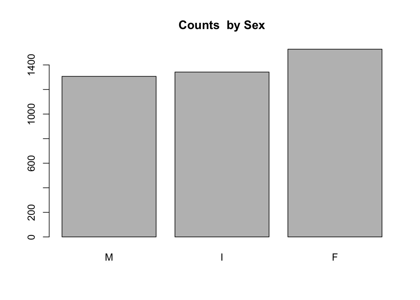
barplot(prop.table(table(a$Sex)), main = "Proportions by Sex")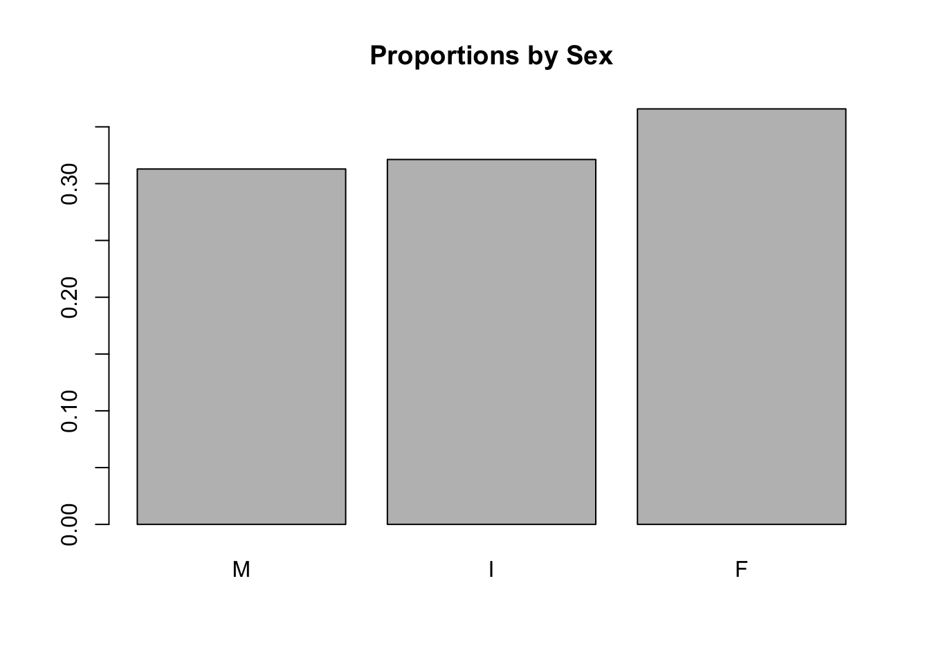
3.6.4 Histograms
Bar plots summarize discrete variables (character of factor); histograms summarize numeric distributions.
hist() chooses a default bin size, counts the observations in that bin, and produces a plot with bars whose heights correspond to the frequency. Histograms are great for visualizing the range and shape of a distribution.
hist(a$Length)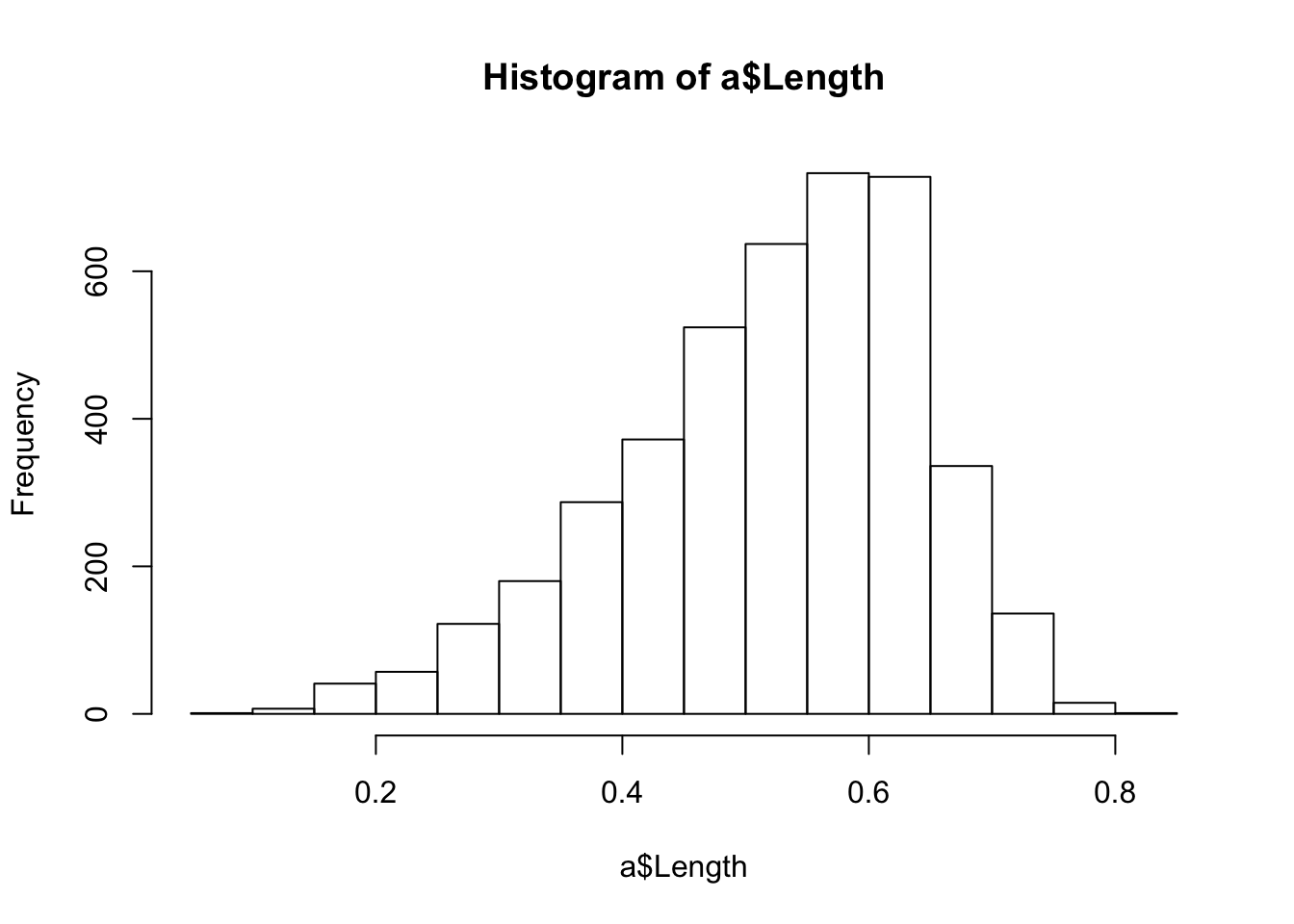
We can see that most abalone, roughly the middle 50% of the distribution, have lengths between about .4 and .7. We can compute quartiles to get this information exactly, either using summary(a) as above, or quantile(a$Length). The default behavior of quantile() is to return quartiles:
quantile(a$Length)## 0% 25% 50% 75% 100%
## 0.075 0.450 0.545 0.615 0.815Remember that quantiles are just percentiles. If we arranged each observation of a$Length from smallest to largest, then 0% would be the minimum and 100% would be the maximum; the first quartile, between .075 and .45, would contain the first 25% of all the observations, while the second quartile would contain the second 25% of all the observations, from .45 to the median, .545; the middle 50% of the distribution would extend from the first quartile, .45, to the third quartile, .615. The middle 50% of the observations can be used to characterize the central tendency of the distribution.
We can adjust the probs argument in the quantile() function to return other percentiles. Here, for example, is how we would get quintiles:
quantile(a$Length, probs = c(0, .2, .4, .6, .8, 1))## 0% 20% 40% 60% 80% 100%
## 0.075 0.425 0.510 0.575 0.625 0.815Let’s include this distributional information on the histogram plot to precisely demarcate the middle 50% of the observations:
hist(a$Length)
abline(v = quantile(a$Length, probs = .25), col="red")
abline(v = quantile(a$Length, probs = .75), col="red")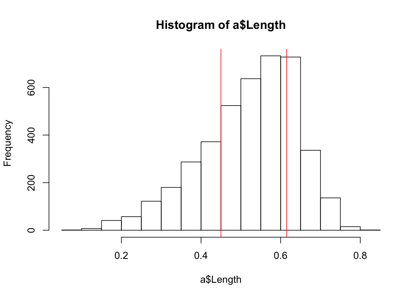
We can decrease the size of the bins using the breaks argument to get finer resolution on this distribution of a$Length:
hist(a$Length, breaks = 100)
abline(v = quantile(a$Length, probs = .25), col="red")
abline(v = quantile(a$Length, probs = .75), col="red")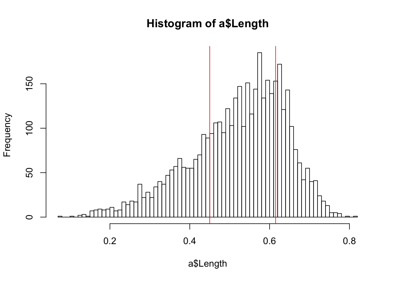
If we want to see what the hist() function is doing in the background we can query it using the “?” command: ?hist. The documentation for histogram indicates that hist() creates an object, consisting in a list, that is used by the function to create the plot. Use str() to look at the components of the list.
str(hist(a$Length, plot = F))## List of 6
## $ breaks : num [1:17] 0.05 0.1 0.15 0.2 0.25 0.3 0.35 0.4 0.45 0.5 ...
## $ counts : int [1:16] 1 7 41 57 122 180 287 372 524 637 ...
## $ density : num [1:16] 0.00479 0.03352 0.19631 0.27292 0.58415 ...
## $ mids : num [1:16] 0.075 0.125 0.175 0.225 0.275 0.325 0.375 0.425 0.475 0.525 ...
## $ xname : chr "a$Length"
## $ equidist: logi TRUE
## - attr(*, "class")= chr "histogram"To subset a list we use double square brackets. In this case, hist(a$Length, plot=F)[[1]] returns the first list item, breaks, which indicates the interval defining each bin.
hist(a$Length, plot=F)[[1]]## [1] 0.05 0.10 0.15 0.20 0.25 0.30 0.35 0.40 0.45 0.50 0.55 0.60 0.65 0.70
## [15] 0.75 0.80 0.85Single square brackets pick out elements from within list items. Thus, hist(a$Length, plot=F)[[1]][1:2] returns the first two elements of the first list item:
hist(a$Length, plot=F)[[1]][1:2]## [1] 0.05 0.10From the documentation for hist() we learn: “If right = TRUE (default), the histogram cells are intervals of the form (a, b], i.e., they include their right-hand endpoint, but not their left one, with the exception of the first cell when include.lowest is TRUE.” include.lowest = T is the default. Thus, the first bin contains all a$Length observations greater than or equal to 0.05 and less than or equal to 0.1.
3.6.5 Density plots
a$Length is a continuous variable, so we should really use a density plot.
plot(density(a$Length))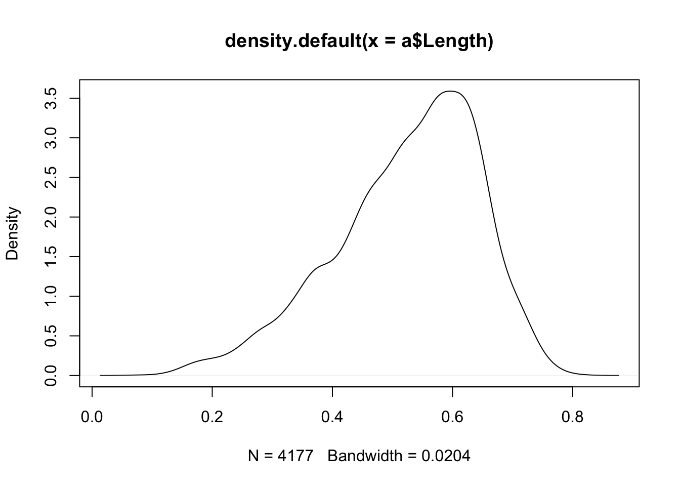
Density plots are basically smoothed histograms, but the density curve does not represent frequencies; instead, the height of the curve represents the probability density function, which can be used to estimate probabilities. For example, the max of the density plot is approximately 3.5 at around x = .6. If we take a small interval around .6—say, .59 to .61—then the height multiplied by the density yields the area under the curve in that region, which is equivalent to the probability for observations occurring in that interval: 3.5 x .02 = 0.07. An interval of the same length in a lower frequency region of the distribution will have a much lower associated probability. For example, the density at x = .4 is about 1.5, so the interval between .39 and .41 would be roughly equivalent to a probability of 1.5 x .02 = 0.03 The area under the density curve is a probability and thus integrates to 1. Read about the details of the algorithm that creates the default density object with?density.
3.6.6 Boxplots
Boxplots are another handy way to summarize, and compare, distributions.
boxplot(a$Length, main="Boxplot of Length", xlab="Length", ylab="Values")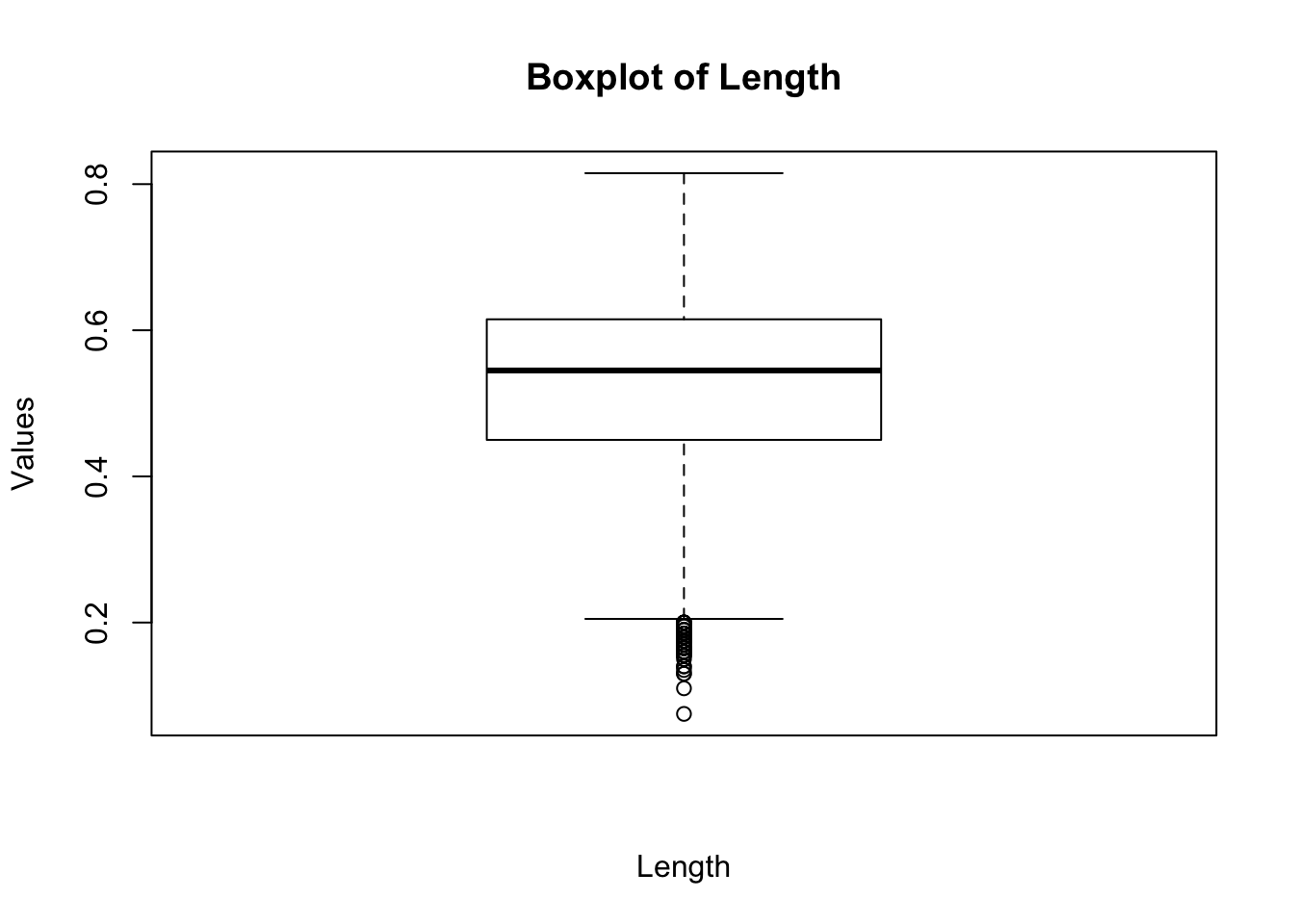
The box in a boxplot represents the interquartile range, or IQR, which contains the observations between the first and third quartiles— the middle 50% of the observations in a distribution.4 The box thus represents the central tendency of the distribution, with its height (or width, depending on the orientation of the box) indicating the spread of the data. The black center line is the median; the edges of the box are known as the “hinges.” The lines extending beyond the hinges are the “whiskers”; they indicate observations that are more extreme than the IQR—less than the first quartile and greater than the third quartile. The whiskers extend 1.5 times the IQR beyond the hinges. If there are no observations that extreme then the whisker extends only as far as the minimum or the maximum. Observations beyond the whiskers—potential outliers—are represented as points. In the above boxplot we can see that there are a number of points smaller than the lower whisker.
As with hist() a call to boxplot() creates an object that we can inspect using str():
str(boxplot(a$Length, plot=F))## List of 6
## $ stats: num [1:5, 1] 0.205 0.45 0.545 0.615 0.815
## $ n : num 4177
## $ conf : num [1:2, 1] 0.541 0.549
## $ out : num [1:49] 0.175 0.17 0.075 0.13 0.11 0.16 0.2 0.165 0.19 0.175 ...
## $ group: num [1:49] 1 1 1 1 1 1 1 1 1 1 ...
## $ names: chr "1"boxplot(a$Length, plot=F)[[1]] in this case returns a five number summary of the distribution: the minimum or the bottom of the lower whisker, the max or the top of the upper whisker, the first and third quartile (the hinges), and the median (the center line).
Boxplots really shine when it comes to comparisons. Here is a boxplot with Sex on the x-axis and Length on the y.
boxplot(a$Length ~ a$Sex, main="Boxplot of Length by Sex",
        xlab="Sex", ylab="Length")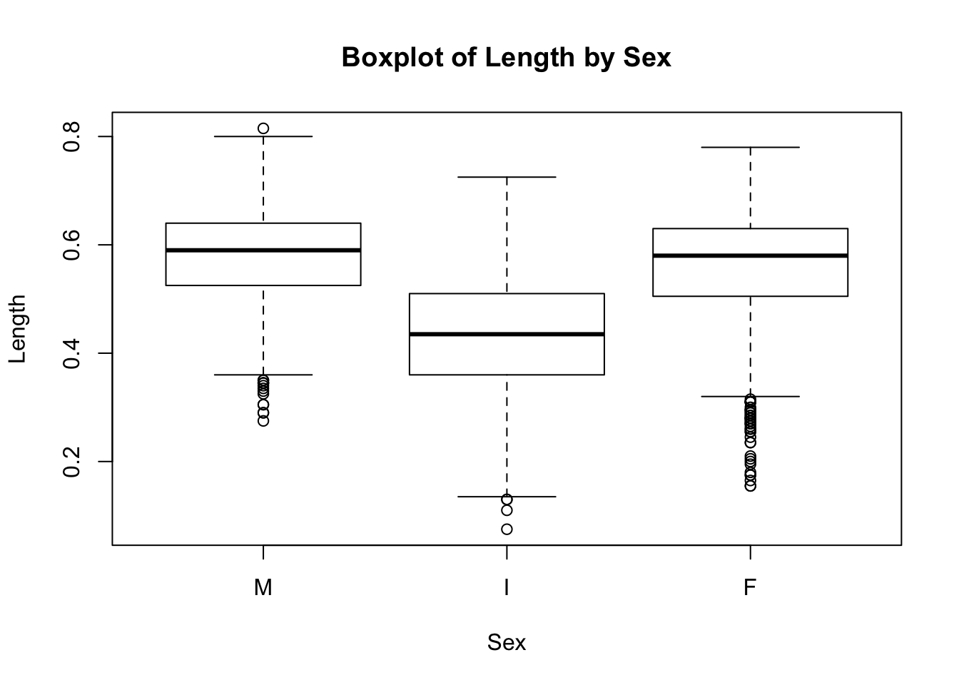
Here we can see that Sex == I accounts for the small lengths that we saw in the first boxplot. While male and female abalone have similar lengths, indeterminates are consistently smaller; the top hinge for Sex == I is below the lower hinge of the other two boxes.
3.6.7 More density plots
Overlain density plots tell a similar story: one of these distributions is not like the other.
plot(density(subset(a, Sex=="M")$Length), xlim = c(0,1), main =
       "Density plot of Length by Sex: \n I  (green), M (black), F (green)")
lines(density(subset(a, Sex=="I")$Length), col=2)
lines(density(subset(a, Sex=="F")$Length), col=3)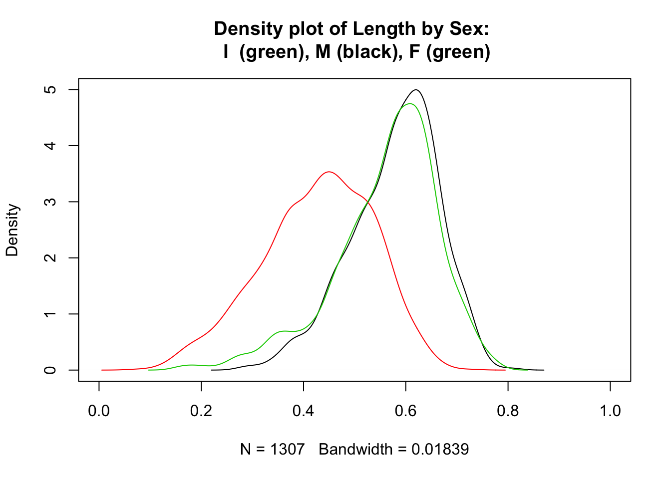
This plot really deserves a legend. Unfortunately, legends are a pain to create in base R—much easier in the ggplot2 package. To create a legend in base R we have to keep track of colors. Black is represented by 1, red by 2 and green by 3. Here is the same plot with a legend.
plot(density(subset(a, Sex=="M")$Length), xlim = c(0,1), main =
       "Density plot of Length by Sex")
lines(density(subset(a, Sex=="I")$Length), col=2)
lines(density(subset(a, Sex=="F")$Length), col=3)
legend("topright",title="Sex", fill=1:3,
       legend =c("M", "I", "F"))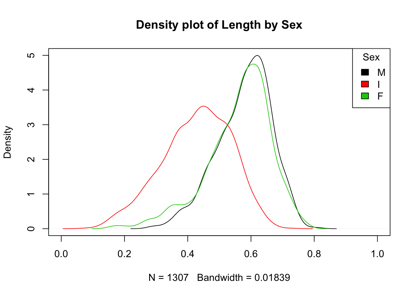
We can also put density plots side by side:
par(mfrow = c(1, 3))
plot(density(subset(a, Sex == "M")$Length), main = "Length for M")
plot(density(subset(a, Sex == "I")$Length), col = 2, main = "Length for I")
plot(density(subset(a, Sex == "F")$Length), col = 3, main = "Length for F")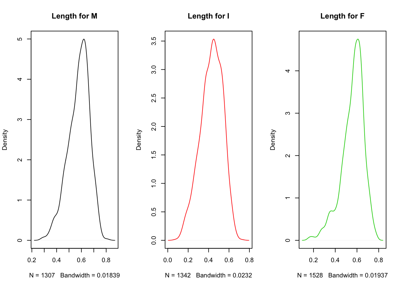
par(mfrow = c(1, 1))We have used the par(mfrow = c(1, 3)) command to tell R how many plots per row we want. Here we specified 3 columns in 1 row; par(mfrow = c(3, 1)) would have arranged 3 rows of plots all in 1 column. It is good practice afterwards to reset this parameter to the default: par(mfrow = c(1, 1)).
Clearly, it is easier to compare distributions when they are all on the same plot (or if they were arranged one above the other rather than side-by-side). Notice also that there are problems here with y-axis scales (they should all have the same scale). These again are formatting challenges handled automatically in ggplot2, so rather than laboring over these base R plots we will return to these issues in the next chapter when we introduce ggplot2.
3.6.8 Scatterplots
Scatterplots are great for showing bivariate relationships between continuous variables. (If one of your variables is a factor, then use a boxplot.) We might expect to find that abalone length and weight are correlated. Here is a scatterplot of length against weight with an ordinary least squares (OLS) line added to summarize the linear relationship:
plot(a$Whole_weight~a$Length,
     main="Relationship between Abalone Length and Weight")
abline(lm(a$Whole_weight~a$Length), col="red")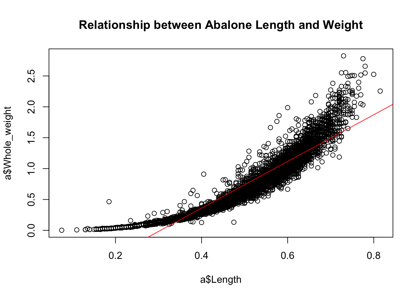
Notice that we have used the lm() function—the main R function for fitting linear models—to add the OLS line. R knows how to extract the intercept and slope from the model object created by lm(). Clearly, however, this is a lousy linear model; the data displays an upward curve that might be better captured with a quadratic term in the model.
A plot showing a nonlinear fit can certainly be produced in base R graphics but is not entirely straightforward: this, task, too, we leave for the next chapter with ggplot2.
One thing we can accomplish fairly easily here is to color the points according to sex. Given the sex differences we’ve observed so far, it might well be the case that they explain this nonlinear relationship. It is, at any rate, worth a look. The following plot colors points by sex, which allows us to visualize how a bivariate relationship—the one between length and weight—varies by sex. Later we will describe this variation across levels of a factor as an interaction. Here length and sex interact to explain weight.
library(scales)
plot(a$Whole_weight~a$Length,
     main="Relationship between Abalone Length and Weight \n varying by Sex",
     col = alpha(as.numeric(a$Sex), 0.5), pch=19)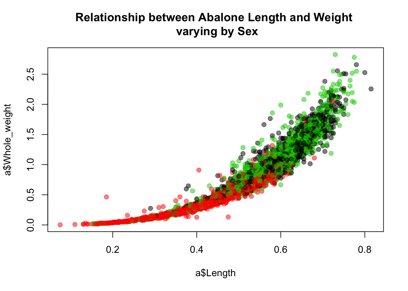
I have added transparency to the points (making the points behind somewhat visible) so we can better see which regions of the distribution are dominated by the different groups.
One possibility for what is going on here—that could be explored further—is that the indeterminate abalone are smaller than males and females, in terms of both length and weight, and that what looks like a nonlinear relationship between length and weight is actually just a linear relationship that varies by group. Plotting these separate fits to investigate this idea is, again, sort of a pain in base R.
We will revisit this topic—displaying linear fits to subsets of the data in the same plot—in the next chapter using ggplot2.
3.6.9 Scatterplot matrix
R has many functions for producing multi-panel plots that display bivariate relationships among all the variables in a data set. Here is one implementation.
pairs(a[,-1])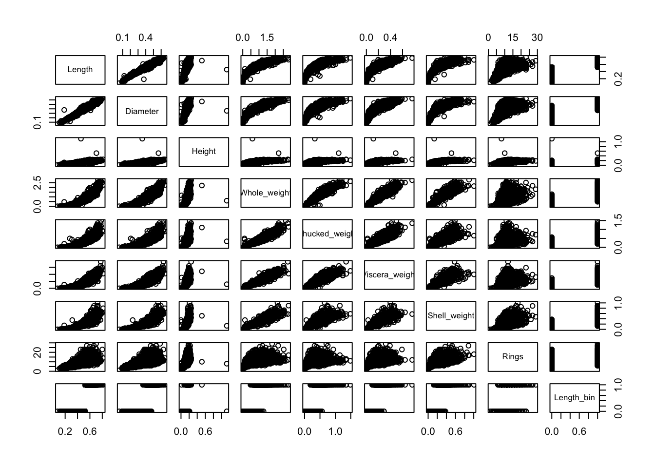
To follow this tutorial, type (or copy and paste) the code examples into your RStudio console and press return. You may, alternatively, open an R script (a .R document) by clicking on the
Filemenu option. SelectNew File>R script. Type (or copy and paste) the code examples into your practice script, then highlight them and presscontrol-returnto run them.↩mtcarscontains information on the design and performance characteristics of older model cars (1973-4).↩If you need information about an R function, you may type “?” in the console followed by the function: for example,
?head. In RStudio this will automatically bring up the documentation for that function under the “Help” tab of the plot pane. The documentation contains comprehensive information about the arguments to the function, details on usage, the values returned, along with examples. In the case ofhead()there are two non-optional arguments:x(data) andn(size), which has a default value of 6. If an argument has a default setting, and you leave it blank, R will use automatically use that default. R functions recognize arguments either by name or position. Thus, because thehead()expects first a data argument then a size argument, these two uses ofhead()are identical:head(mtcars, n = 10)andhead(mtcars, 10).↩The hinges are actually “versions” of the first and third quartiles. See the documentation for
boxplot.stats()for details.↩