Chapter 11 Microbial Ecology
"If I could do it all over again and re-live my vision in the 21st century, I would be a microbial ecologist.
Ten billion bacteria live in a gram of ordinary soil: a mere pinch held between thumb and forefinger. They represent thousands of species, almost none of which are known to science.
Into that world I would go with the aid of modern microscopy and molecular anlaysis. I would cut my way through clonal forest sprawled across grains of sand, travel in an imagined submarine through drops of water proportionately the size of lakes, and track predators and prey in order to discover new life ways and alien food webs.
All this, and I need venture no farther than ten paces outside my laboratory building. The jaguars, the ants, and the orchids would still occupy distant forests in all their splendor, but now they would be joined by an even stranger and vastly more complex living world virtually without end."
– E.O. Wilson
11.1 r/K Selection Theory
The driving idea behind this is that species selection drives evolution to its maximal growth rate (i.e., the r strategy) or its maximum carrying capacity (i.e., the K strategy). This idea was popular in the 70s era of macro ecology, yet the irony was that no studies were done to validate the model.
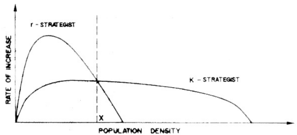
Figure 11.1: r/K Species
r-selected species are opportunists: they have a high growth rate, many offspring, a less crowded niche, and a lower survivorship.
This is in contrast to K-selected species: specialists that have a low growth rate, less offspring, and strong competitors.
11.1.1 Some strategies for r/K selection theory
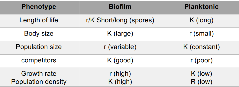
Figure 11.2: Some Strategies for r/K Selection Theory
11.2 Microbial Diversity
The term species richness refers to the number of species within a group of individuals. This “group” can be acquired by sampling colonies, sequences, and now, even single cells from samples!
11.2.1 Operational taxonomic unit
The unit of diversity is defined by method, not the species concept.
The type of operations available is defined by the available data: operational taxonomic units also circumvent the traditional species definition as a unit of diversity and can be used with culture-based data.
Furthermore, one can also trace a phylogenetic (i.e., core gene) or functional (i.e., auxillary gene) gene marker using operational taxonomic units. Such data is also amenable to molecular data (i.e., sequencing the 16s rRNA gene with a 98% similarity).
However, do note that sequencing a protein encoding gene is a sensitive process - it leads to an additional base pair being added and also has limited universality.
11.2.2 Simpson’s diversity index
Simpson’s diversity index \(S\) is denoted by:
\[\begin{equation} S = 1 - \frac{n}{N^2} \end{equation}\]
Where:
- \(N\) is the number of organisms from all species
- \(n\) is the species richness (i.e., the number of species)
Hence, when \(1 - D\) increases, the value of the diversity index also increases.
The index also measures the true diversity in not just the number, but also proportional distribution of species.
11.2.3 Shannon index
The Shannon index \(H'\) is denoted by:
\[\begin{equation} H' = -\sum_{i = 1}^{R}p_i \times \log{(p_i)} \end{equation}\]
This measures the entropy (i.e., uncertainty) in the data (i.e., when sampling a population, what is the uncertainty in predicting the next individual); note that:
- \(R\) is the species richness
- \(p_i\) is the proportional abundance of \(i\)
11.2.4 Species evenness
The species evenness \(J'\) is denoted by:
\[\begin{equation} J' = \frac{H'}{H'_{\text{max}}} \end{equation}\]
Note that \(H'\) assumes an even distribution of species
11.2.5 Why do diversity indices indicate?
The above indices all indicate how many species are in a sample, the species’ distribution throughout the community, and also the discovery (i.e., new diversity).
It is believed that systems with high diversities are robust to disturbance and permanent change due to genetic redundancy. Such systems are also more productive and leads to optimization and innovation.
In redundant systems, this means that species share niches and have multiple interactions, metabolisms, and behaviors that achieve the same outcome.
11.3 Keystone Species
Dominant species are species whose influences on their community are because of their large numbers.
Foundation species influence their community by changing their environment.
Keystone species are species whose influence on their ecosystem and community are disproportional to their abundances.
While keystone species are keystone (no pun intended) to their community’s structure as they maintain their integrity and presence over time, they also tend to be high in the food web. The interactions of keystone species are often through trophic interactions.
11.4 Community Ecology
A community is a group of interacting organisms in a pre-defined time and space.
Community ecology is the study of change in the structure and variation of a community or between communities over time.
Alpha diversity studies community diversity within a habitat.
Beta diversity studies community diversity between habitats.
Gamma diversity studies large scale landscape diversities (i.e., alpha and beta diversity).
11.5 Biogeography
This is the study of the geographical distribution of species - in this context, diversity is determined in terms of speciation, dispersal, and extinction.
If one can understand how past and current environments have shaped the above three factors for determining diversity, then we would understand the biogeographical forces shaping communities.
Note that biogeography simultaneously ranges from fine to large spatial scales.
Vicariance is the separation of a continuously distributed ancestral population or species into separate populations due to the development of a geographical or an ecological barrier. Unfortunately, the mechanisms of vicariance is still poorly understood.
11.5.1 Z slopes
A Z slope models the strength of the relationship between species richness and area.
A high Z value suggests that species richness is highly responsive to area. (e.g., genetic bottlenecks, speciation, population size, genetic redundancy, carrying capacity, etc).
A contiguous habitat is one where there are bridges between habitats.
11.6 Succession
This is the directional and predictable change that a community undergoes over time - the shifts in succession are usually in the presence and abundance of species.
While succession generally focuses on plant species, all species are subjected to succession nonetheless.
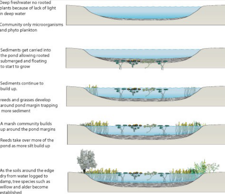
Figure 11.3: Succession on a Macro Scale
Succession is also driven by the interaction between biotic and abiotic factors (e.g., as each species colonize an environment, they change the environmetn around them to be more suitable for other species).
11.6.1 Types of succession
Primary succession occurs when a new habitat is colonized. The rate of succession here is a little bit slower; habitats need to be developed and niches need to be formed.
Secondary succession occurs after some sort of disturbance. Disturbances reduce the succession stage of a community and over time, establishes a new climax community.
The climax community is the stable, end state community from succession. It should be stable (obviously) and define the habitat (e.g., Prairie grasses or kelp forests).
11.6.2 Succession experiments
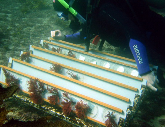
Figure 11.4: Field Succession Experiments
These usually take the form of field assays - above is an example.
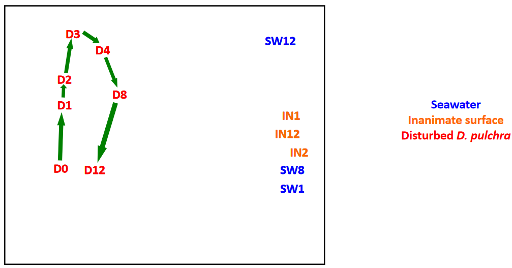
Figure 11.5: Bacterial Succession on Seaweed
Nevertheless, the colonization of seaweed is also a process of succession - natural antibiotics found in seaweed may also play a potential role in guiding succession.
11.7 Landscape Ecology
In the past, ecologists have observed abiotic and biotic influences on populations over time and space. However, spatial heterogeneity was ignored as it was difficult to resolve.
However, technological and statistical methods were developed in 2005 (e.g., GPS). Scale is one of the key themes in landscape ecology that allows questions of population, habitat, dispersal, and conservation to be simultaneously addressed.
11.7.1 Corridors and stepping stones
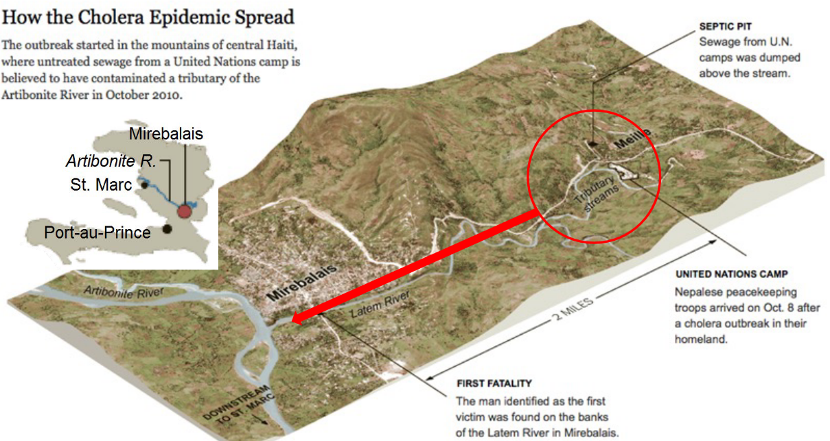
Figure 11.6: Corridors in the Haitian Earthquake
Advanced imaging and mapping techniques are unable to resolve patchiness in microbial populations - hence, corridors and stepping stones are also useful for tracking the spread of diseases: a feat that can be done by tracking the host (i.e., corridors and stepping stones have the potential to track the source of an infection).
11.8 Indicator Species
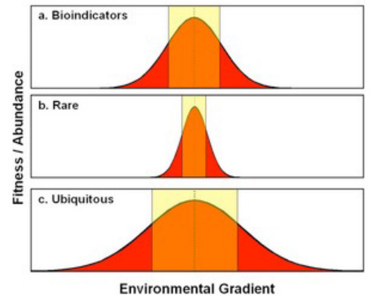
Figure 11.7: Fitness of Several Types of Indicator
Bioindicators can be biological processes, species, or communities. A change in the size of any one of the latter three aspects can also indicate a change in an environmental process. While these three aspects are usually anthropogenic, they can also be natural.
An indicator species will hence have physiology that is reponsive to some environmental variable (e.g., canaries in coal mines, frog spawn and pollution levels, freshwater shrimp in lakes, etc).
11.8.1 Microbial indicators
Microbes can also be great indicators of biological processes and as indicator species themselves. Microbes can be counted directly (i.e., CFU counts) or indirectly (i.e., biomarker molecules).
Biomarker molecules are diagnostic molecules for the presence of an organism: for instance, fatty acids, DNA, and proteins.
11.9 Why are Microbial Systems so Amenable to Ecology?
Microbial systems have / are:
- A large population size
- A short generation time
- Genetic manipulation
- Readily sampled
- Experimentally tractable
- Different modes of genetic inheritance