Chapter 6 Regression
Linear regression is a directed association between two (or more) metric variables. The goal of linear regression is to predict (estimate) unknown values, and determine the quality of the prediction (clarification of variance).
In the context of regression, we call the independent variable the predictor, and the dependent variable is criterion (predicted value).
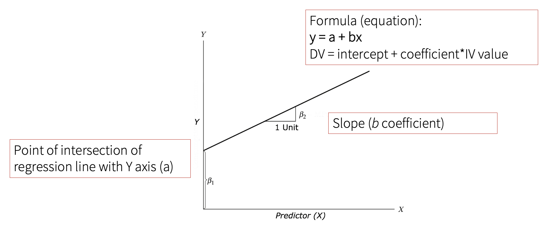
Regression is basically a straight line that assigns a point on the Y axis to each point on the X axis. It is determined by the intersection with the X axis (i.e., mean of Y), and slope coefficient b.
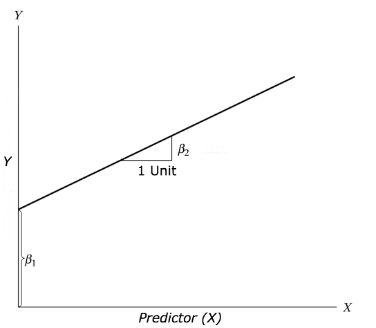
The formula for regression is as follows:
\(y = a + bx\)
Regression represents the data best when all data points deviate as little as possible from the straight line. To calculate this, for each data point the distance to the straight line is determined, the distance is squared and all distances are summed up.
Goodness of fit measure R2
The regression line represent the relationship between IV and DV very well when the estimation error is small, which is indicated by high variance.
To show how well our model represents the relationship, we report the adjusted R Square (R2). It is called “adjusted” because it takes into account the number of IVs and the sample size.
6.1 Regression in R
The contact hypothesis (Allport, 1954) assumes that contact with members of an “outgroup” (based on nationality, religion, etc.) can reduce prejudice. Using the dataset Prejudice_Refugees (largely representative sample, N = 765), we can see see whether there’s really a correlation.
Research question: Is there a connection between contact with refugees (Contact_Refugees) and negative experiences with refugees (Negative_experience_refugees)?
First, we load the necessary packages. You will need to package haven for loading the .sav dataset and for the regression, we will be package called car.
Then we need to load the dataset Prejudice_Refugeesto R:
Now we can use the function lm() to calculate the regression model and display it with the summary() function.
regression_model <- lm(Negative_experiences_refugees ~ Contact_refugees,
data=prejudice_refugees)
summary(regression_model)
The output should look like this:
Call:
lm(formula = Negative_experiences_refugees ~ Contact_refugees,
    data = prejudice_refugees)

Residuals:
    Min      1Q  Median      3Q     Max
-3.7345 -1.4732  0.2115  1.2655  4.1575

Coefficients:
                 Estimate Std. Error t value Pr(>|t|)
(Intercept)       2.52716    0.16632  15.194   <2e-16 ***
Contact_refugees  0.31534    0.03664   8.606   <2e-16 ***
---
Signif. codes:  0 ‘***’ 0.001 ‘**’ 0.01 ‘*’ 0.05 ‘.’ 0.1 ‘ ’ 1

Residual standard error: 1.838 on 763 degrees of freedom
Multiple R-squared:  0.08847,   Adjusted R-squared:  0.08728
F-statistic: 74.06 on 1 and 763 DF,  p-value: < 2.2e-16
To interpret this, we first take a look at the adjusted R square, which in this case equals to 0.08728. Therefore, we can conclude that 8,7 % of the variance of negative experience toward refugees is explained by personal contact with refugees.
Then, we need to take a look at the estimate for the contact_refugees (our IV). We can see that it equals 0.31534, which means that the regression line increases by 0.31534 units, i.e., this is the slope of the regression line (b).
The intercept estimate tells us that at the value 2.52716 the regression line intersects the Y axis (a).
Therefore, the regression equation for this example would be:
\(Y = 2,527 + 0,315*X\)
Formally, we could interpret the result as follows:
The regression shows significant positive relationship of personal contact with refugees on negative personal experiences with refugees (b = 0.315, p < .001). In other words, the more contact a person has with refugees, the more negative personal experiences a person has.
6.2 Multiple regression
Multiple regression includes not one, but several predictor (IVs) to improve the prediction of the DV. It is an extension of the regression equation.
Each regression weight (beta weight) describes how strongly the predictor is related to the criterion - but in relation to all other predictors! The regression coefficient thus reflects the specific predictive power, which is only given by this predictor and no other (adjusted).
6.3 Mutiple regression in R
Using the dataset Prejudice_Refugees, we can now calculate a multiple regression with contact with refugees (Contact_refugees) as IV and prejudice towards refugees as a DV (Prejudice_refugees), while we control for the political ideology (Ideology).
The code would look like this:
multiple_regression <- lm(Prejudice_refugees ~ Contact_refugees+Ideology,
data=prejudice_refugees)

summary(multiple_regression)
The output:
Call:
lm(formula = Prejudice_refugees ~ Contact_refugees + Ideology,
    data = prejudice_refugees)

Residuals:
   Min     1Q Median     3Q    Max
-5.924 -1.203 -0.068  1.256  5.554

Coefficients:
                 Estimate Std. Error t value Pr(>|t|)
(Intercept)       0.49125    0.24004   2.047    0.041 *
Contact_refugees  0.06307    0.03452   1.827    0.068 .
Ideology          0.89195    0.04731  18.853   <2e-16 ***
---
Signif. codes:  0 ‘***’ 0.001 ‘**’ 0.01 ‘*’ 0.05 ‘.’ 0.1 ‘ ’ 1

Residual standard error: 1.73 on 762 degrees of freedom
Multiple R-squared:  0.3225,    Adjusted R-squared:  0.3207
F-statistic: 181.4 on 2 and 762 DF,  p-value: < 2.2e-16
We can see that 32.7 % of the variance in prejudice toward refugees is explained by personal contact with refugees AND political ideology (adjusted R-squared).
When we compare of different coefficients within the regression, the higher the estimate value, the greater the effect. Consequently, political ideology has a greater influence on prejudices against refugees than personal contact with refugees.
If we add variable political ideology to the model, we can see that personal contact with refugees no longer significantly influences prejudice against refugees (p > 0.05). However, political ideology does have a significant influence on prejudices towards refugees (b = 0.89, p < 0.001). Since the estimate coefficient is positive, stronger “right-wing” ideology leads to higher prejudice against refugees.
6.4 Participation Exercise 6
Calculate a simple linear regression predicting how positive personal experiences with refugees as an IV (Positive_experiences_refugees) influence prejudice towards refugees as a DV (Prejudice_refugees).
- Load the package
havenand load the datasetPrejudice_refugees.savto R:
- Install and load the package
car.
- Using the
lm()function, calculate a simple linear regression predicting how positive personal experiences with refugees as an IV (Positive_experiences_refugees) influence prejudice towards refugees as a DV (Prejudice_refugees). You can do that by adjusting the following code:
regression_model <- lm(Dependentvariable ~ IndependentVariable,
data=DatasetName)

summary(regression_model)
Copy paste the output to a Word file (or add a screenshot), and interpret the results (Adjusted R-Squared, estimates & p-values).
Repeat the analysis with political ideology (
Ideology) as a control variable:
multiple_regression <- lm(Dependentvariable ~ IndependentVariable+ControlVariable,
data=DatasetName)

summary(multiple_regression)
Copy paste the output to a Word file (or add a screenshot), and interpret the results (Adjusted R-Squared, estimates & p-values). Explain which variable has the greatest influence.
Upload the R script & Word file to folder Participation Exercise 6 on Moodle.