Chapter 4 T-Test
4.1 Testing hypotheses
When creating statistical hypotheses, we make a distinction between two key concepts:
the null hypothesis (H0): which suggests that there is no effect or relationship, and
the alternative hypothesis: which suggests that an effect or relationship does exist
Inferential statistics tests whether the alternative hypothesis is likely to be true.
For example, if we want to explore the relationship between education and political interest, we can pose these hypotheses:
H0= There is no relationship between education and political interest.
Halternative= There is a relationship between education and political interest.
To check the association, we calculate the error probability (= probability that H0 applies): This is shown with a p-value (probability) in statistical results.
4.1.1 Significance levels: p-value
P-value tells us what is the probability that our results were produced by chance (random).
In the social sciences, a p-value below 0.05 (i.e., a lower probability of error than 5%; p < .05) is usually considered “significant”.
Based on the p-value, we either accept (p < .05), or reject (p > .05) our hypothesis.
If p-value is below 0.05, we reject the null hypothesis (H0).

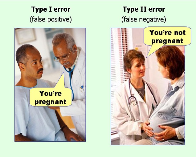
4.1.2 Types of errors
When we draw conclusions about the “real” world, we have to be careful because there are two types of errors which can occur:
- Type 1 error (Alpha error): We reject the null hypothesis, although in reality it is correct
- Type 2 error (Beta error): We assume the null hypothesis, even though in reality it is false
4.2 T-test
T-test is an analysis for mean value comparison. We use t-test in cases where the independent variable is nominal and dependent variable is metric to see if there are differences between their means.
T-test is applied in cases where the the independent variable has two characteristics. The dependent variable (effect) is measured and compared for both values.
Example research questions for which the t-test could be used:
- Are viewers of Scream 1 (group 1) more afraid than viewers of Scream 2 (group 2)?
- Are newspaper readers (group 1) older or younger than the non-readers (group 2)?
- Are there significant differences between men (group 1) and women (group 2) regarding internet use?
There are two types of t-test:
1. T-test for independent samples (two independent groups)
Independent variable is different in two groups (violent film seen vs. violent film not seen)
- Compares two values that are independent of each other
- There are two experimental groups and each participant participated in only one
RQ: Does a difference in the independent variable lead to a significant difference in the dependent variable?
Examples:
Do viewers of violent films differ from viewers of not violent films in their subjective aggressiveness?
Are men more aggressive than women after watching a violent film?
2. T-test for dependent samples (two dependent measuring points)
Several persons are examined at two measurement times with the same test instrument
- Compares two mean values that are related (repeated measurement)
- There are two test conditions and each participant participated in both
RQ: Have the mean values changed between the two measurement times?
Examples:
- Investigation of subjective levels of aggression (dependent variable) BEFORE and AFTER watching a violent film (independent variable)
4.2.1 T-test for Independent Samples
T-test is a parametric test, meaning that certain prerequisites or requirements must be fulfilled. If these prerequisites are violated, then it’s more likely that we will arrive at wrong conclusions.
For the independent t-test, the requirements are groups of equal size with equal variance and normally distributed variables.
When the variances are the same, having groups of different sizes is generally less of an issue. However, if there are significant differences in both the sizes and variances of the samples, it’s more likely that incorrect conclusions will be drawn. This problem persists even when the samples are of equal size but the data does not follow a normal distribution and the variances are unequal. The assumption that the dependent variable is normally distributed is equivalent to saying it follows a Gaussian curve.
In R, we can use descriptive statistics or the Kolmogorov-Smirnov test to assess normality.
4.2.1.1 Kolmogorov-Smirnov-Test
If p-value is smaller than 0.05, the test is significant and we can say that data are not normally distributed.
Let’s test the normal distribution for the variable selfesteem_1 in data set Self_esteem.
ks.test(Self_esteem$selfesteem_1,
        "pnorm",
        mean=mean(Self_esteem$selfesteem_1),
        sd=sd(Self_esteem$selfesteem_1))
>
Asymptotic one-sample Kolmogorov-Smirnov test
data: Self_esteem$selfesteem_1
D = 0.22983, p-value = 1.758e-06
alternative hypothesis: two-sidedThe output tells us that the p-value is p-value = 1.758e-06. That means that p = 1,758 * 10-6, which equals to 0,000001758. Therefore, p < 0,001, meaning that the test is significant. In other words, the data is not normally distributed.
4.2.1.2 Spider Example
Imagine the following test situation. We have conducted an experiment with two experiment groups. In group 1 (n = 12), 12 participants saw a real spider and then their fear was measured. In group 2 (n = 12), other 12 participants saw a picture of a spider and then their fear was measured.
Our RQ is: Are acute anxiety states among people with arachnophobia triggered only by real spiders or is a picture of the spider enough?
First, we need to formulate our hypotheses.
Null hypothesis H0: There is no difference between the two groups (picture vs. real spider).
- In other words, the two researched groups (samples) come from a population whose parameters µ1 and µ2 (mean values) are identical.
Alternative hypothesis H1: There is a difference between the two groups (picture vs. real spider).
Let’s test these hypotheses using the SpiderBG data set and the following code:
    Welch Two Sample t-test

data:  spiderBG$Anxiety by spiderBG$Group
t = -1.6813, df = 21.385, p-value = 0.1072
alternative hypothesis: true difference in means between group 0 and group 1 is not equal to 0
95 percent confidence interval:
 -15.648641   1.648641
sample estimates:
mean in group 0 mean in group 1
             40              47
R calculates Welch T-test by default (instead of the Student’s t-test, which is calculated by SPSS for example). Advantage: Welch’s t-test also works with unequal variances.
In this case, p = 0.107, which means that p is larger than 0.05 and thus we cannot reject the H0. In other words, there is no mean difference between the groups.
In order to be able to report the results, we also need descriptive statics for the tested variables. For that we can use function describeBy from the package psych. If you do not have this package downloaded use install.packages("psych"). Do not forget that everytime you want to use the package, you need to first load it using library(psych).
 Descriptive statistics by group
group: 0
   vars  n mean   sd median trimmed   mad min max range skew kurtosis   se
X1    1 12   40 9.29     40      40 11.12  25  55    30    0    -1.39 2.68
------------------------------------------------------------------------------------------------------------------------------------------------------
group: 1
   vars  n mean    sd median trimmed   mad min max range  skew kurtosis   se
X1    1 12   47 11.03     50    46.9 14.83  30  65    35 -0.01    -1.46 3.18
Interpretation:
The participants who had direct contact with the spider were on average more afraid (M = 47.00, SD = 11.03) than those who looked at only one spider image (M = 40.00, SD = 9.29). However, this difference is not significant, because the probability of error is greater than 5%, t(21.385) = -1.68, p = 0.107.
4.2.2 T-test for Dependent Samples
The t-test for dependent samples compares two mean values that are related (repeated measurement). In other words, there are two test conditions and each participant participated in both.
4.2.2.1 Spider Example 2
Imagine the following test situation. We have conducted an experiment with 15 participants (n = 15). Each of the 15 participants was shown a real spider and at another time a picture of the spider. Each time the fear of the participants was measured.
Our RQ is: Are acute anxiety states among people with arachnophobia triggered only by real spiders or is a picture of the spider enough?
We will use the SpiderRM data set this time and include the parameter paired = TRUE in the function to tell R that we want to calculate the t-test for dependent samples.
    Paired t-test

data:  spiderRM$picture and spiderRM$real
t = -2.3245, df = 11, p-value = 0.04026
alternative hypothesis: true mean difference is not equal to 0
95 percent confidence interval:
 -23.3626091  -0.6373909
sample estimates:
mean difference
            -12
We can see that p-value = 0.040, which means that p < 0.05. In this case, we can thus reject the H0 and conclude that there is a significant mean difference between the groups. In order to be able to report the results, we again need also descriptive statics for the tested variables. However, if we want to use the describeBy function again, we need to run individually for each variable because unlike the independent sample test, we do not have a grouping variable.
> describeBy(spiderRM$picture)
   vars  n mean   sd median trimmed   mad min max range skew kurtosis   se
X1    1 12   40 9.29     40      40 11.12  25  55    30    0    -1.39 2.68

> describeBy(spiderRM$real)
   vars  n mean    sd median trimmed   mad min max range skew kurtosis   se
X1    1 12   52 14.92     50    51.4 15.57  30  80    50 0.28    -1.12 4.31
Interpretation:
On average, the participants were more afraid of direct contact with the spider (M = 52.00, SD = 14.92) than when looking at a spider picture (M = 40.00, SD = 9.29). The difference between the two groups is significant, t(11) = -2.32, p = 0.04.
4.3 Participation exercise 4
- Open the Self_esteem data set
- Calculate the mean value for self-esteem index (high values should mean high self-esteem, you need to recode some variables before computing an index)
- You would like to know whether the self-esteem in the sample differs significantly between informatics and journalism (Publizistik) students. Based on that formulate the null hypothesis and the alternative hypothesis (in a Word Document).
- Use the independent sample t-test to check whether the mean value for self-esteem differs significantly between informatics and journalism students.
- Copy the results in the Word document and interpret the results.
- Upload the Word/PDF file and the R script file on Moodle
4.3.1 Step-by-step instructions
Create a new RScript in your STADA project File -> New File -> R Script
Load the necessary packages, in this case
psych,havenanddplyrLoad the dataset Self_esteem using the
read_sav()functionFirst, you need to compute an index for self-esteem so that high values mean high self-esteem. Open the dataset in R and read what each item stands for and decide whether it needs to be recoded or not, e.g.,:

There are 3 items that need to be recoded. Recode them by adjusting this code snippet:
dataset_name <- dataset_name %>%
  mutate(
    new_variable_rec = case_when(
      old_variable == 1 ~ 7,
      old_variable == 2 ~ 6,
      old_variable == 3 ~ 5,
      old_variable == 4 ~ 4,
      old_variable == 5 ~ 3,
      old_variable == 6 ~ 2,
      old_variable == 7 ~ 1,
      TRUE ~ old_variable
    ))
or like this (7 is the highest value):
Compute the self-esteem index by adjusting the following code snippet:
IMPORTANT: Enter the recoded variables for those items that had to be recoded!
- You would like to know whether the self-esteem in the sample differs significantly between informatics and journalism (Publizistik) students. Based on that formulate the null hypothesis and the alternative hypothesis (in a Word Document or as comments in the RScript using #).
- Use the independent sample t-test to check whether the mean value for self-esteem differs significantly between informatics and journalism students. Use the function
t.test()and put in the dependent variable (selfesteem_index) and indepedent variable (study_field). - Use the function describeBy to calculate the descriptives.
- Save the R Script and then copy the results in the Word document and interpret the results.
- Upload the Word/PDF file and the R script file on Moodle