Chapter 3 Data Management

3.1 Recoding variables

3.1.1 Example - Grades

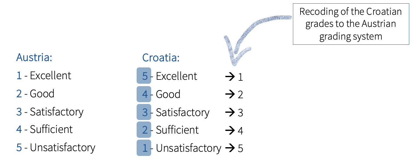
A student has grades from an Austrian university as well as from a Croatian university and wants to calculate their grade average. However, the grading scheme in the two countries is different (i.e., reversed). In order to calculate the average, the student needs to recode the grades from one country.

Austria	Croatia
1 - Excellent	5 - Excellent
2 - Good	4 - Good
3 - Satisfactory	3 - Satisfactory
4 - Sufficient	2 - Sufficient
5 - Unsatisfactory	1 - Unsatisfactory

The recoding would look like this:

Let’s try to do it in R!

First, we will create a dataset with the grades from Austria (AT) and Croatia (HR):

AT <- c(2,1,3,2,4,1,2,2,5,3)
HR <- c(4,3,5,2,4,4,5,1,2,5)

grades <- data.frame(AT, HR)

This dataset includes grades of 10 people from each country. We can visualize how the grade distribution looks like per country:

barplot(table(grades$AT), main = "AT Scores", xlab = "AT", ylab = "Frequency", col = "skyblue")

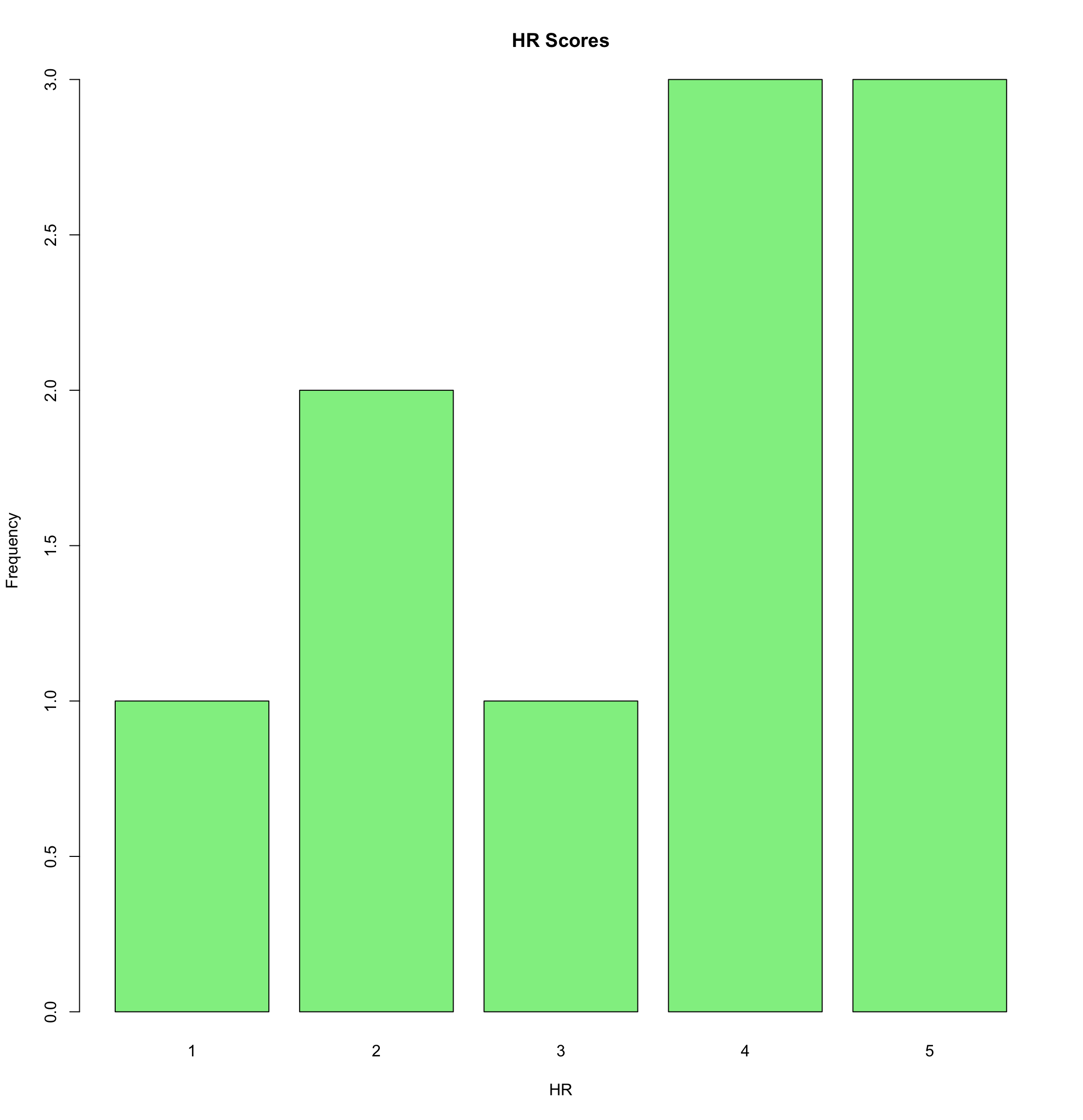
barplot(table(grades$HR), main = "HR Scores", xlab = "HR", ylab = "Frequency", col = "lightgreen")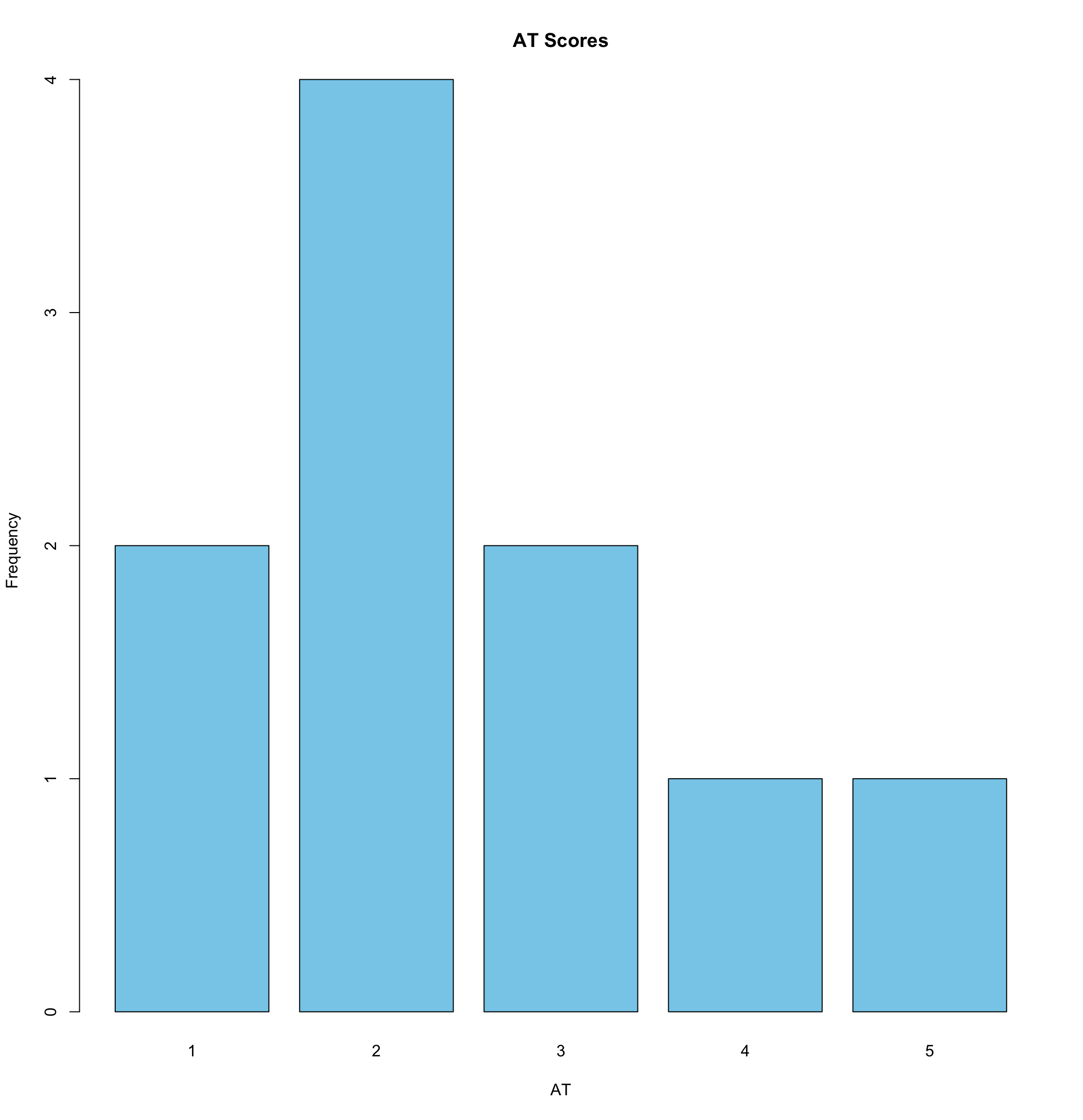

We can also calculate the mean for each country:

mean(grades$AT)
#[1] 2.5

mean(grades$HR)
#[1] 3.5

From an Austrian perspective, it looks like students from Croatia have on average worse grades than Austrian students. However, because the same grade means different things in both countries, we need to recode the values of one country to be able to compare them.

We have two main options how to recode the Croatian grades.

Option 1: We can use the dplyr package and function mutate:

library(dplyr)
grades <- grades %>%
  mutate(HR_rec = recode(HR, `1` = 5, `2` = 4, `3` = 3, `4` = 2, `5` = 1))

Option 2: Another way to recode variables which are reverse (like our grades), is to subtract the original values from the maximum value plus one. In our example, the maximum value is 5. Therefore, we can simply subtract the original values from 6 (i.e., 6-5 = 1; 6-4 = 2; 6-3 = 3; 6-2 = 4; 6-1= 5):

grades$HR_recoded <- 6 - grades$HR

When we now display the dataset, we can see that both options yielded the same results, i.e., we know have two more columns HR_rec (option 1) and HR_recoded (option 2) with the same values. You can thus decide by yourself which method you want to use.

> grades
   AT HR HR_recoded HR_rec
1   2  4          2      2
2   1  3          3      3
3   3  5          1      1
4   2  2          4      4
5   4  4          2      2
6   1  4          2      2
7   2  5          1      1
8   2  1          5      5
9   5  2          4      4
10  3  5          1      1

If we now take a look at the mean values of the grades of students from both countries, we will see that they are the same (2.5).

mean(grades$AT)
mean(grades$HR_rec)

3.1.2 Example - Newspaper use

Sometimes we want to recode variables in a different way than to just reverse them. Let’s look at the dataset Media_use.sav. First, we need to load the dataset:

library(haven)
Media_use <- read_sav("Media_use.sav")

We are interested in how many people from our dataset read newspapers. The variable newspaper_use is an ordinal variable with values “1 - never”, “2 - rarely”, “3 - sometimes”, “4 - often”. Therefore, to see how many people read newspapers (no matter how often), and how many don’t, we need to recode the values so that 1 = 0, and all the other variables are 1.

Option 1: We can again use the dplyr package and function mutate:

Media_use <- Media_use %>%
  mutate(newspaper_use_rec = case_when(
    newspaper_use == 1 ~ 0, # 1 to 0
    TRUE ~ 1  # All other valzes (2, 3, and 4) to 1
  ))

Option 2: Another option is to use the function ifelse() from the base R:

Media_use$newspaper_use_recoded <- ifelse(Media_use$newspaper_use == 1, 0, 1)

In this code, ifelse() is used to check each value of newspaper_use. If the value is 1, it recodes that as 0. For any other value, it assigns a 1, indicating that the person reads newspapers to some extent.

3.2 Selecting cases

We select cases (i.e., filter) when we do not want to consider all cases in the analysis, but only some of the cases (e.g., only certain age group, only specific education levels etc.). Then, only the selected cases are included in further analyses.

For example, we can filter only those people who read newspapers. For that we can use function filter from package dplyr. The following code creates a new dataset called Filtered_data that contains only data for those people who read newspapers (i.e., they have value 1 for variable newspaper_use_rec).

Filtered_data <- Media_use %>%
  filter(newspaper_use_rec == 1)

3.3 Computing an index

Some variables are not directly observable and need to be measured with number of items (i.e., latent variables), such person’s self-esteem. In order to combine all items into one construct, we create a mean index.

Load the dataset self_esteem from Moodle and inspect it:

self_esteem <- read_sav("self_esteem.sav")
self_esteem

First we need to define missing values. Missing values occur, for example, when participants do not answer a question. These are often saved as a numerical value (e.g., 99). If these values are not excluded in advance, they would distort the mean index. So we have to tell R that 99 means “no information”. The following code uses the function mutate_at from dplyr package to replace values of 99 with NA (missing values) in all columns starting with “selfesteem”.

self_esteem <- self_esteem %>%
  mutate_at(vars(starts_with("selfesteem")), ~na_if(., 99))

We can see that self-esteem was measured using 6 different statements. However, not all statements have the same polarity and thus needs to be recoded:

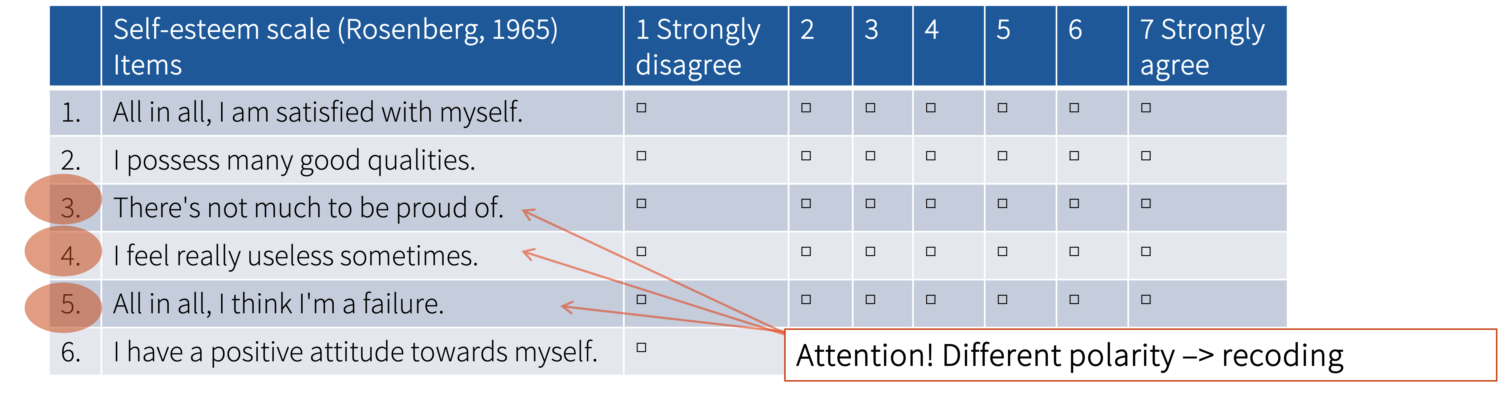
To recode the items we can again create new columns and subtract the values of the original variables from the maximum value plus 1 (i.e., from 8 in this case because the highest value is 7).

self_esteem$selfesteem_3_rec <- 8 - self_esteem$selfesteem_3
self_esteem$selfesteem_4_rec <- 8 - self_esteem$selfesteem_4
self_esteem$selfesteem_5_rec <- 8 - self_esteem$selfesteem_5

Now that all variables are coded in the same direction (i.e, high value means high self-esteem), we can calculate the mean index, which we can then use as an indicator of a person’s self-esteem.

self_esteem <- self_esteem %>%
  mutate(
    selfesteem_index = rowMeans(select(., c(
      selfesteem_3_rec, 
      selfesteem_4_rec, 
      selfesteem_5_rec, 
      selfesteem_1, 
      selfesteem_2, 
      selfesteem_6)), na.rm = TRUE)
  )

Now we can look at the mean of this index, which would tell us the average level of self-esteem in our dataset:

mean(self_esteem$selfesteem_index)
# [1] 5.772727

3.4 Participation Exercise 3

In this exercise, you need to:

define missing values
recode a variable
compute an index

3.4.1 Step-by-step instructions

Create a new RScript in your STADA project File -> New File -> R Script
Load the necessary packages, in this case haven and dplyr
Load the dataset Mobile_phone_use using the read_sav() function
We will be working with variable loneliness, which is measured using 5-point scale with the following items:
- V_7 I often feel alone.
- V_8 I often think I am no longer close to anyone.
- V_9 I often feel close to other people.
- V_10 Sometimes I feel like nobody really knows me.
- V_11 I often feel isolated from others.
- V_12 Most of the time I think that there are people who really understand me.
- V_13 There are people in my life to whom I can turn to.
Define missing values using the following code:

Mobile_phone_use <- Mobile_phone_use %>%
  mutate_at(vars(starts_with("v_")), ~na_if(., 99))

Carefully read all the items and decide which ones need to be recoded. To recode them use either function mutate from the dplyr package or subtract the values from the highest values +1. If you decide to use mutate, follow the following template:

dataset_name <- dataset_name %>%
  mutate(
    new_variable_rec = case_when( # rec means recoded; this code makes a new column, i.e., variable in the dataset
      old_variable == 1 ~ 5,
      old_variable == 2 ~ 4,
      old_variable == 3 ~ 3,
      old_variable == 4 ~ 2,
      old_variable == 5 ~ 1,
      TRUE ~ old_variable
    ))

Compute a mean value index and using the function mutate from the dplyr package and name it loneliness_index.
Calculate the mean value and standard deviation of the new index.