UE STADA
2024-03-08
Chapter 1 Getting started with R
This is an online resource developed to support students attending the UE STADA class at the University of Vienna, Austria.
You can use the chapter overview on the left to skip through the content.
In this session, we will answer the following questions:
- What is R?
- What is RStudio?
- How do I download R and RStudio?
- How do I use RStudio?
- What are R packages?
- How do I get started with R?
1.1 What is R?
R is a programming language used mostly for statistical computing and data visualization.
Why are we using R and not other software such as SPSS?
- Unlike many statistical softwares, R is open-source and completely free
- R is a very powerful and versatile tool for both statistics and visualization
- Analyses conducted in R are transparent, reproducible and easy to share
- R has a large and active community, offering extensive resources for learning and problem-solving
- Learning a programming language enhances your digital skills
1.2 What is RStudio?
In this class we will be working in RStudio. The following picture illustrates the difference between R and RStudio:
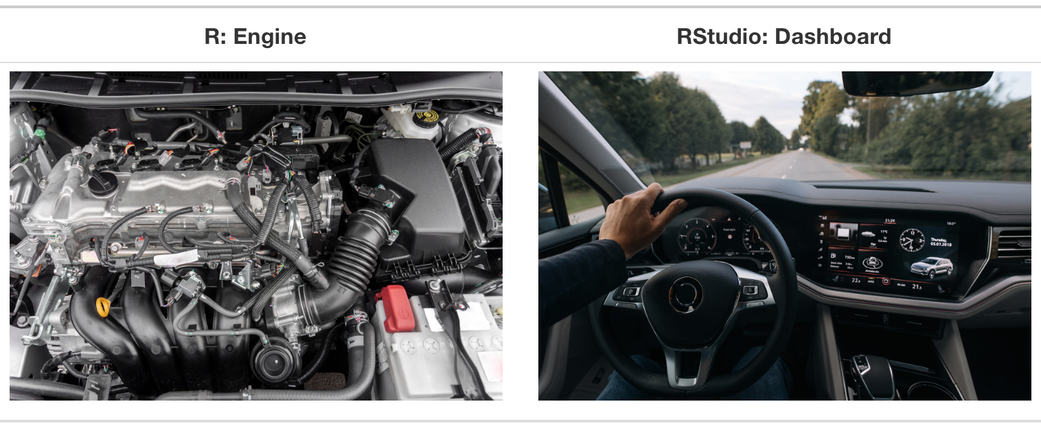
R as the Engine:
- Core functionality: Just as the engine is the heart of a car, powering its operation and driving its performance, R is the core of statistical computing and graphics. It’s the fundamental software that executes the statistical analysis and data manipulation.
- Essential but not user-friendly: An engine is essential for a car to function, but it’s not something you interact with directly in a user-friendly manner. Similarly, R is a powerful and essential tool for data analysis, but it can be complex and less accessible, especially for beginners or those not familiar with programming.
RStudio as the dashboard:
- Interface for Interaction: The dashboard in a car provides the controls and indicators that allow the driver to operate and monitor the vehicle effectively. RStudio serves a similar purpose for R; it’s the interface through which users interact with R. It provides a more user-friendly environment to write code, visualize data, and manage projects.
- Enhanced usability and accessibility: Just as a dashboard makes it easier to drive a car by organizing controls and information efficiently, RStudio enhances the usability of R. It offers features like code auto-completion, syntax highlighting, and tabbed windows for scripts, visual output, and file management, making the process of coding in R more accessible and efficient.
Just as a car needs both an engine and a dashboard to function effectively, R and RStudio are complementary. RStudio is designed specifically to work with R and relies on R for its statistical computing power.
In summary, R is the underlying power and functionality, essential for data analysis tasks, while RStudio is the interface that makes the power of R more accessible, organized, and user-friendly, much like a car’s dashboard facilitates the operation and control of the car’s engine.
1.3 How do I download R and RStudio?
To be able to work with R and complete both the participation exercises and homework assignments for the UE STADA class, you will need to download and install both R and RStudio to your computer.
IMPORTANT: First, you need to download and install R. Only afterwards you can install RStudio.
Step 1: Download and install R
If you are a Windows user: Click on “Download R for Windows”, then click on “base”, then click “on the Download link”Download R-4.3.3 for Windows”. If you are macOS user: Click on “Download R for macOS”, then under “Latest release:” click on
- “R-4.3.3-arm64.pkg” - if you have a MacBook with the Apple silicon (M1/M2/M3) chip
- “R-4.3.3-x86_64.pkg” - if you have a MacBook with the Intell chip
How to find out which chip your MacBook has: Click on the in the upper left corner of your Mac → Click on “About this Mac” →The first line in the pop-up window tells you what kind of chip you have
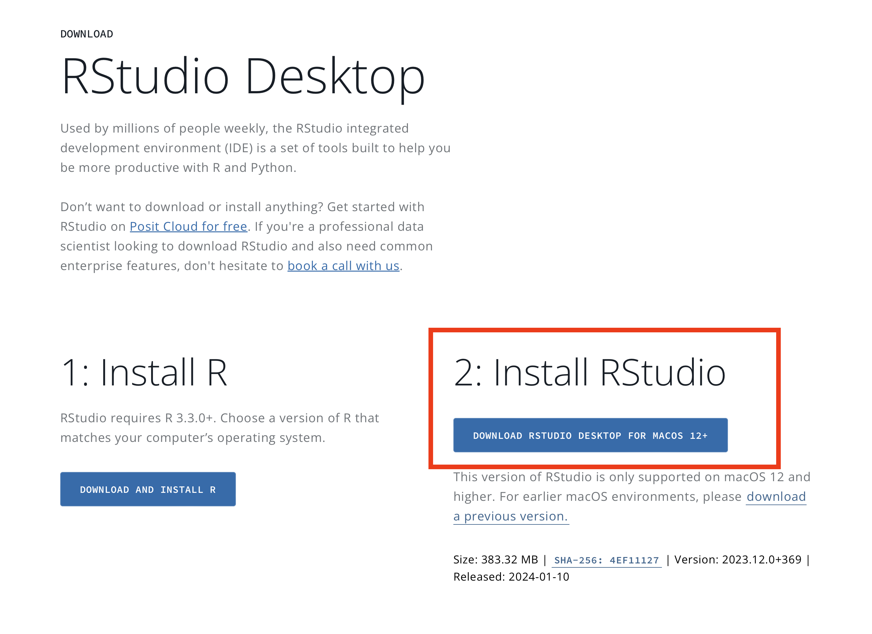
Step 2: Download and install RStudio
- Go to https://posit.co/download/rstudio-desktop/
- Click on “Install RStudio for [your operating system]”
- Alternatively, scroll down to “All Installers and Tarballs”, choose the version of RStudio that corresponds to your operating systems and click on the download file
- Follow the instructions of your computer to install the program
Step-by-step tutorials to downloading and installing R and RStudio:
Windows
MacOS
1.4 How do I use RStudio?
If you successfully followed the instructions, you should have these two new programs on your computer:

To work with R, we will always use the RStudio. Therefore, you always
need to open this program:
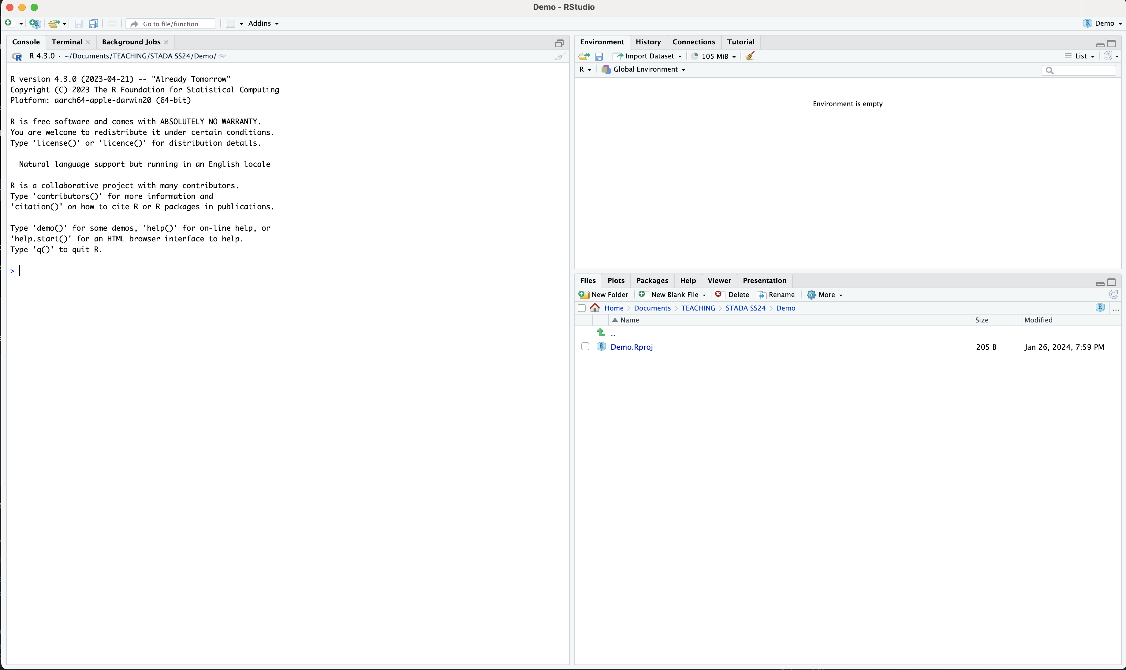
Once you open RStudio, you should see something like this:
TIP: You can change the appearance of the RStudio and your code. To do this, go to “Edit” → “Setting” → “Appearance” → Choose which “Editor theme” you like and click “Apply”
1.4.1 RStudio panes
When you first open the RStudio, you will see three panes that divide
the screen: 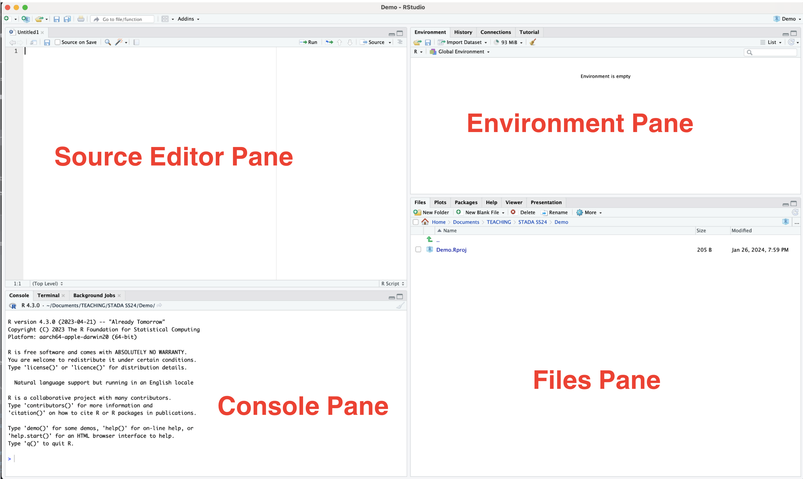
Console Pane:
- The Console Pane in RStudio is where you can directly interact with R. It’s like having a conversation with the R program. When you type a command here and press Enter, R executes that command and shows you the result right in this pane. It’s also where messages, warnings, and errors from R are displayed. Think of it as the place where you talk to R and see its immediate responses.
- For example, if we write
10+2to the console and hit enter, we will immediately get a result:
Files Pane:
- The Files Pane is essentially a file manager within RStudio. It shows you all the files and folders in your current working directory (the folder where R is currently operating). You can think of it as a window into your computer’s file system, but focused on the location relevant to your R project. Here, you can open, rename, delete, or view the files, just like you would in a typical file explorer on your computer. This pane makes it easy to navigate and manage the files you’re working with in R.
- In this pane you can also switch to different tabs such as:
- Plots: Here you would see the results of your visualizations (e.g., graphs)
- Packages: An overview of installed R packages
- Help: Here you can find explanations and guidelines for different functions and topics
Environment Pane:
- The Environment Pane is like a display cabinet where you can see all the objects (like datasets, variables, functions) that you have created or are currently available in your R session. Every time you create a new variable or load a dataset, it appears in this pane. This helps you keep track of what data and objects you have on hand and their current state. You can think of it as a summary or inventory of the tools and materials you’re working with in your R project.
Your panes might be displayed in a different order than on the screenshots. You can change their order/placement by clicking “Edit” → “Setting” → “Pane Layout”
It may not be visible at the moment but there is also a 4th pane in the RStudio interface:
- Source Editor Pane
- The Source Editor Pane is the main area where you write, view, and manage your code. It is like a digital notepad where you write and tweak your R code. It’s color-coded to make your code easy to read and understand. You can run your code directly from this pane and the results will be displayed in the Console. It’s also great for keeping multiple code files open and organized with tabs, almost like having several notepads open at once.
1.5 R Basics
Before we start working with R in RStudio, you need to have basic understanding of a few topics.
1.5.1 R Operators
R has many different operators, which are fundamental for working with data. These operators help you change, examine, and organize data, making it easier to do calculations and manage your information.
For example, we can use arithmetic operators to perform calculations:
+Addition- Adds two numbers.
Example:
- Adds two numbers.
-Subtraction- Subtracts the right-hand operand from the left-hand operand.
Example:
- Subtracts the right-hand operand from the left-hand operand.
*Multiplication- Multiplies two numbers.
Example:
- Multiplies two numbers.
/Division- Divides the left-hand operand by the right-hand operand.
Example:
- Divides the left-hand operand by the right-hand operand.
^Exponentiation- Raises the left-hand operand to the power of the right-hand
operand.
Example:
- Raises the left-hand operand to the power of the right-hand
operand.
Basic Arithmetic Operators
| Operator | Description | Example | Result |
|---|---|---|---|
+ |
Addition | 3 + 2 |
5 |
- |
Subtraction | 5 - 2 |
3 |
* |
Multiplication | 4 * 3 |
12 |
/ |
Division | 10 / 2 |
5 |
^ |
Exponentiation | 3 ^ 2 |
9 |
Assignment Operators
<-Assignment- Assigns value on the right to the object on the left.
Example:
=can also be used for assignment, but<-is preferred.Example:
- Assigns value on the right to the object on the left.
Assigning values to an object is a very common operation in R. In this context, object can be a lot of different things, such as a dataset, number(s) or a character(s), result of some computation, a function etc.
Essentially, an object is a broad label for various components involved in your data analysis. Objects are particularly useful for holding results that you might want to utilize in subsequent stages of analysis. Let’s take a look at the following example:
In this instance, I’ve established an object named favoriteFruit and
set “Apple” as its value. “Apple” is a text string, so it’s enclosed in
"".
Now we can ask R to display the value of an object in the console by
simply typing the object’s name, favoriteFruit, and pressing Enter ↵.
Important: R is case-sensitive! If I would say favouritefruit, I would get an error.
#Comment- As you might have noticed in the examples, we can use
#to add comments to our code.
Example:
- As you might have noticed in the examples, we can use
1.5.2 R Functions
Functions are like helpful tools that perform specific tasks or calculations on data. You give a function some input, and it processes that input according to a set of instructions, then gives back a result or performs an action.
To illustrate this, let’s expand our fruit collection from the previous
example. To create objects holding multiple items, we make use of the
c() function, which stands for ‘concatenate’.
# Expanding my fruit collection
favoriteFruit <- c("Apple",
                   "Banana",
                   "Watermelon",
                   "Strawberry",
                   "Kiwi",
                   "Peach")

# Displaying all my favorite fruits
favoriteFruitTo concatenate values into a single object, it’s crucial to use a comma
, to separate each value. If we forget the comma, R will return an
error.
In this case, c() is an R function.
Another example of a function could be sum(), which adds all input
numbers together.
During this course, you will learn many different functions that will allow you to perform statistical operations in R.
1.5.3 R Objects
There are many different types of R objects. Here are some of the basic ones:
1. Vectors
Vectors are sequences of values of the same type (e.g., numbers).
2. Lists
A list can hold elements of different types, including numbers, , characters, etc.
3. Matrices
A matrix is a table composed of rows and columns containing only numerical values.
4. Data Frames
A data frame is a table where each column contains values of one variable and each row contains one set of values from each column.
1.5.4 Types of R files
In R, there are several types of files you can work with, each with a different purpose.
In this class we will mostly be working with the following file types:
.R Files: These are script files containing R code. They are plain text files where you write and save your R commands and functions.
.RData or .Rda Files: These files store R data objects, such as vectors, matrices, or data frames. They are used for saving and loading workspace data.
.Rproj Files: R Project files. They represent a working directory for R and include user-specific settings. Opening an .Rproj file sets the working directory and environment to that specific project.
.csv Files: Though not specific to R, CSV (Comma-Separated Values) files are commonly used to store tabular data and can be read into and written from R.
1.5.5 Packages
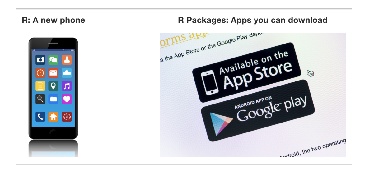
Packages in R are collections of functions, data, and compiled code that are bundled together. They extend the functionality of R, allowing you to perform additional tasks that aren’t available in the base R software. Think of them as add-ons or plugins that you can install to do specific types of analysis or data manipulation.
You can think of packages as apps on your phone. Using this analogy, your phone would the R - it has some basic functions but it can do much more if you download some apps (=packages) (Ismay & Kim, 2023):
When you first start using the RStudio, it will only have one package
called base, which includes the very basic functions of R. If you
would like to download and use some other packages, you always need to
first install them and then, everytime you’d like to use them, you
need to load them.
As explained by Phillips (2018), you could also imagine that packages
are lightbulbs. If you want to get some light in your home, you first
need to install a lightbulb (=install package). Then, whenever you want
to use the lightbulb, you need to go and turn it on (=load package):
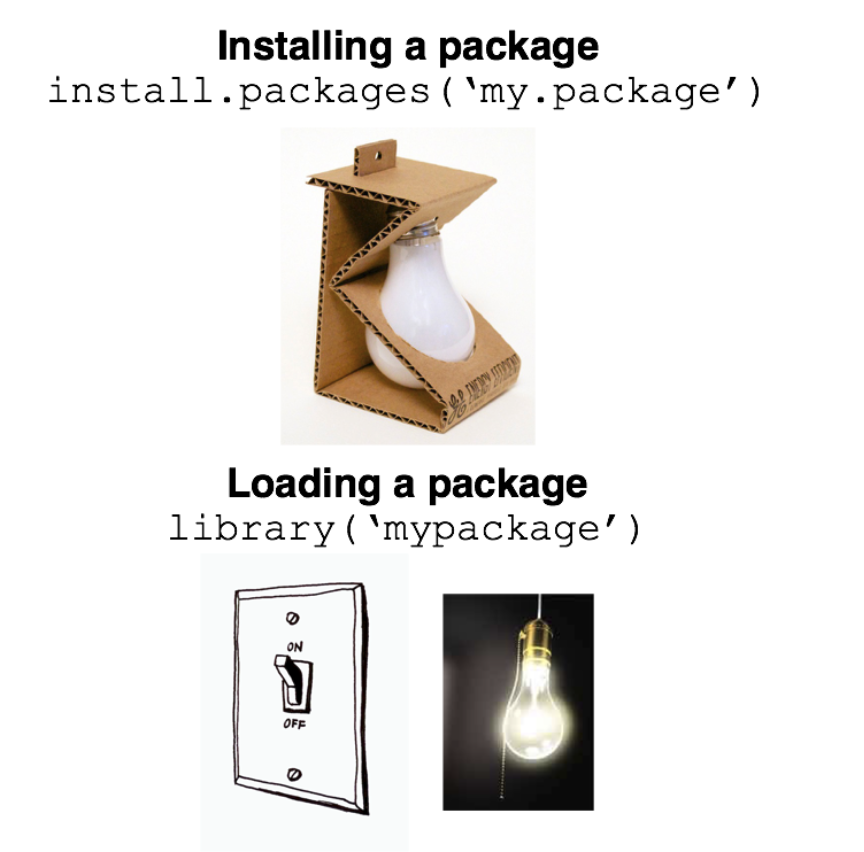
To install a package use:
To load a package use:
1.6 My first project in RStudio (Participation Exercise 1)
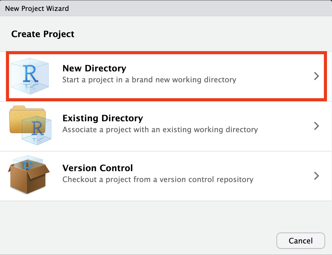
When you open RStudio for the first time, you will need to create a new project. R projects are dedicated environments where we can keep all scripts (files containing our code), data sets and outputs of our analysis, such as plots and tables. To create a new project go to File → New Project.
Click on New Directory
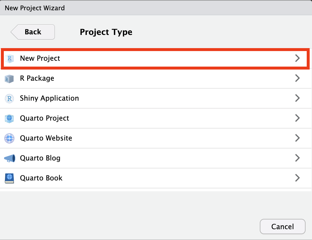
Click on New Project
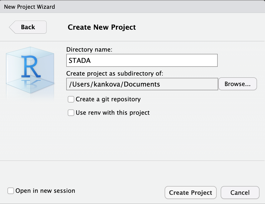
Name your working directory STADA. R will create a new folder for your STADA project, select where you want it to be (e.g., Documents folder). Then click on Create Project.
5. Go to File -> New File -> R Script

Now we want to create new data set using the script based on the answers of 5 survey participants:

First, we will create the variables using the assignment operator and the
c()function. Use the following code, the values for the two participants are already there, replace the three dots with the rest of the values based on the table above:
gender <- c("Man","Woman", ...)
age <- c(21,18, ...)
education <- c("Graduation","Secondary certificate", ...)
newspaper_use <- c("rarely","sometimes", ...)
socialmedia_Facebook <- c("Yes","No", ...)
socialmedia_Instagram <-c("Yes","Yes"...)
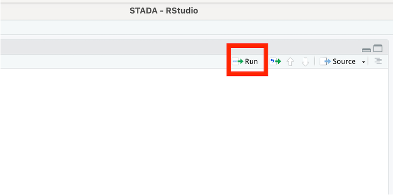
socialmedia_WhatsApp <-c("No","Yes", ...)To run the code in R you can either put the cursor on the line of the command and then click the Run button or just press CTRL-Enter (Windows)/ Cmd-Enter (MacOS). You can also select the whole code and run it all at once.
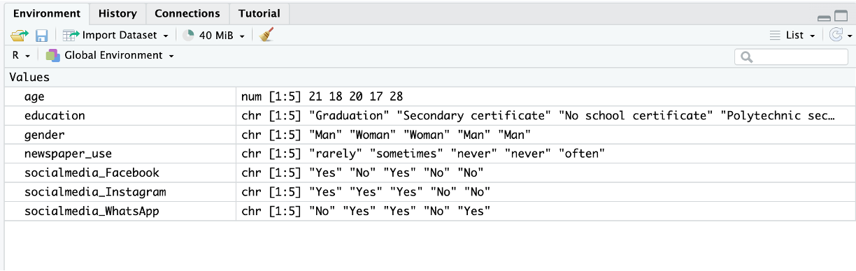
Once you run the code, the new variables should appear in your environment pane:
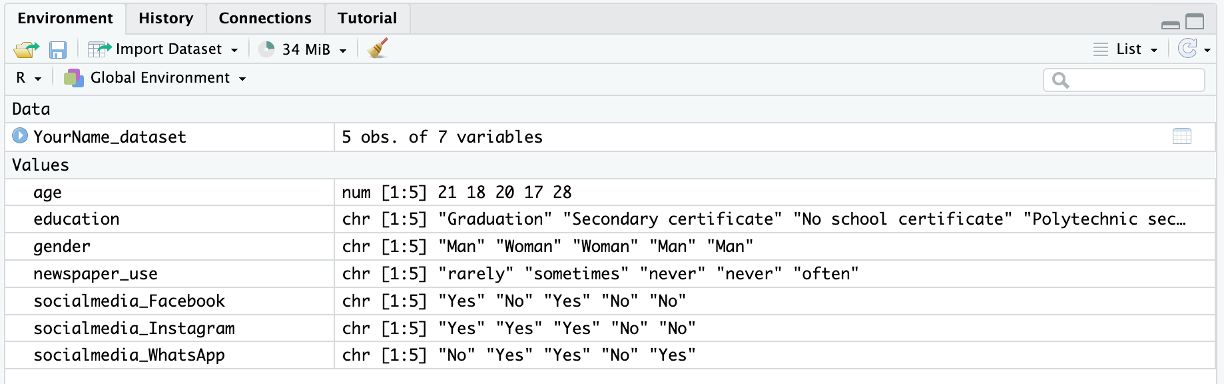
Now we want to take these variables and their values and create a new data set. We will use the
data.frame()function for that. Copy the following code snippet and change the name of the dataset based on the format, and replace the three dots with all the other variables that we want in our data set.
- Once you run the code, the new data set should also appear in your
environment pane:
If you click on it, a new tab opens next to your script in the source
editor pane displaying the data set: 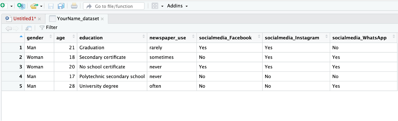
- Now let’s try to use the
head()function, which is used to quickly view the first few rows of a data set or vector.
The output should appear in your console and look like this:

- Next, we would like to add a new column to our data set called pid
(participant id). To do operations with specific columns, we use the
$sign. The following code adds a new column called pid to the dataset. It also specifies that the pid values should go from 1 to the number of rows in our data set. Once you run it, check if the new column was added using thehead()function.
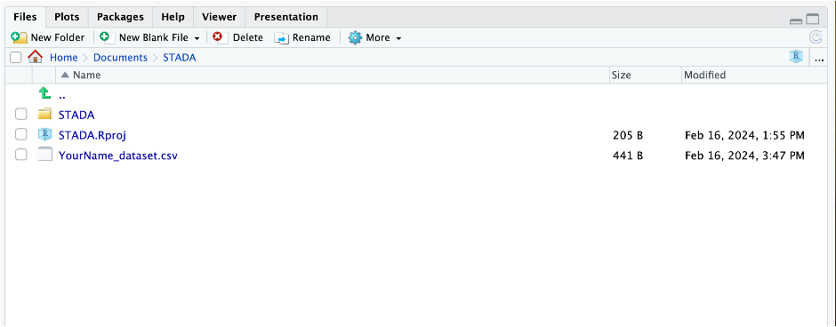
- Lastly, we want to save our new data set and RScript. To save the dataset as a .csv file, run the following code:
R will automatically save the file into your working directory (your
STADA file). You will be able to see it in the files pane as well:
- We also want to save our R script → Click on the Save button in the R script tab. Once you click on it, new window will open. Name the file as YourName_PE1.R and save it to your STADA file.

1.7 References
Ismay, C., & Kim, A. Y. (2023). Statistical Inference via Data Science. https://moderndive.com
Field, A., Miles, J., & Field, Zoë (2012). Discovering statistics using R. London: SAGE Publications.
Phillips, N. D. (2018). YaRrr! The Pirate’s Guide to R. https://bookdown.org/ndphillips/YaRrr/