Chapter 5 Chi-square Test & Correlation

5.1 Chi-square test

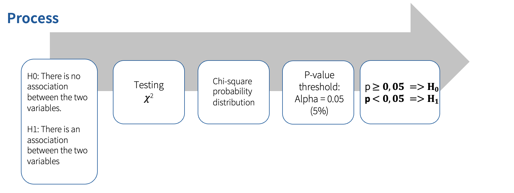
The Chi-square test analyzes whether there is an association between two categorical variables (those are non-metric variables that have nominal or ordinal scale). The observed frequencies are compared with theoretically expected frequencies. The strength and direction of the correlation are then determined.

We can have a chi-square test for

• 2x2 table = two categorical variables, each with two categories i.e., nominal

• 3x3 table

5.2 Requirements for conducting the chi-square analysis

• The variables are categorical (nominal or ordinal scale)
• The samples are independent of each other (dependent samples, e.g., repeated measurements, cannot be examined with the Chi-square test).
• All expected frequencies should be greater than 0 and not more than 20% should be less than 5.
  • If the last condition is violated:
    • Fisher’s Exact test can be applied to a 2x2 table
    • If there are more than 2x2 values, merge or collect more data
    • Otherwise not interpretable

5.3 Chi-Square in R

We can use the chi-square analysis to answer the research question question “Is there a connection between gender and the smoking behavior of the respondents?”

First, we need to load the dataset Gender_behavior.sav to R using the read_sav() function from the haven package:

First load the haven package:

library(haven)

Then load the dataset into R:

gender_behavior <- read_sav("Gender_behavior.sav")

Then we can use the CrossTable function from the gmodels package to calculate the chi-square:

First install and load the package:

install.packages("gmodels")
library(gmodels)

Then calculate the chi-square:

CrossTable(gender_behavior$Gender, gender_behavior$Smoking_behavior,
chisq = TRUE, fisher = TRUE, expected = TRUE, sresid = TRUE, format = "SPSS")

The result should look like this:

   Cell Contents
|-------------------------|
|                   Count |
|         Expected Values |
| Chi-square contribution |
|             Row Percent |
|          Column Percent |
|           Total Percent |
|            Std Residual |
|-------------------------|

Total Observations in Table:  100 

                       | gender_behavior$Smoking_behavior 
gender_behavior$Gender |        0  |        1  | Row Total | 
-----------------------|-----------|-----------|-----------|
                     1 |       36  |       14  |       50  | 
                       |   24.000  |   26.000  |           | 
                       |    6.000  |    5.538  |           | 
                       |   72.000% |   28.000% |   50.000% | 
                       |   75.000% |   26.923% |           | 
                       |   36.000% |   14.000% |           | 
                       |    2.449  |   -2.353  |           | 
-----------------------|-----------|-----------|-----------|
                     2 |       12  |       38  |       50  | 
                       |   24.000  |   26.000  |           | 
                       |    6.000  |    5.538  |           | 
                       |   24.000% |   76.000% |   50.000% | 
                       |   25.000% |   73.077% |           | 
                       |   12.000% |   38.000% |           | 
                       |   -2.449  |    2.353  |           | 
-----------------------|-----------|-----------|-----------|
          Column Total |       48  |       52  |      100  | 
                       |   48.000% |   52.000% |           | 
-----------------------|-----------|-----------|-----------|

 
Statistics for All Table Factors


Pearson's Chi-squared test 
------------------------------------------------------------
Chi^2 =  23.07692     d.f. =  1     p =  1.556476e-06 

Pearson's Chi-squared test with Yates' continuity correction 
------------------------------------------------------------
Chi^2 =  21.19391     d.f. =  1     p =  4.150813e-06 

 
Fisher's Exact Test for Count Data
------------------------------------------------------------
Sample estimate odds ratio:  7.941543 

Alternative hypothesis: true odds ratio is not equal to 1
p =  2.756371e-06 
95% confidence interval:  3.06007 22.06963 

Alternative hypothesis: true odds ratio is less than 1
p =  0.9999998 
95% confidence interval:  0 18.90682 

Alternative hypothesis: true odds ratio is greater than 1
p =  1.378185e-06 
95% confidence interval:  3.494611 Inf 


 
       Minimum expected frequency: 24 
       

Based on the table, we can see that. for example:

• 72 % of all men are non-smokers

• 28 % of all men are smokers

• 75 % of all non-smokers are men

• 25 % of all non-smokers are women

The chi-square test results indicate a significant relationship between gender and smoking behavior (𝛘 2(1) = 23.08, p < .001, N = 100).

With this test, we have found out that there is indeed a statistically significant relationship between smoking behavior and gender, but how strong is this relationship? For that, we need to measure the measures of the strength of the association:

• Phi (ϕ): suitable for 2x2 tables
• Cramer’s V: used for all table sizes

To calculate these coefficients in R, we need to follow these steps:

1. Calculate the Chi-square value and save it as an object

Chi_Square_Test <- chisq.test(gender_behavior$Gender, gender_behavior$Smoking_behavior)

2. Extract the observed values and save them as an object

Observed_values <- Chi_Square_Test$observed

3. Calculation of the Phi coefficient for 2x2 table

if (all(dim(Observed_values) == c(2, 2))) {
  phi <- sqrt(Chi_Square_Test$statistic / sum(Observed_values))
  print(paste("Phi (φ):", phi))} 

4. Calculation of the Cramer’s V

n <- sum(Observed_values)
min_dim <- min(dim(Observed_values))
cramers_v <- sqrt(Chi_Square_Test$statistic / (n * (min_dim - 1)))
 
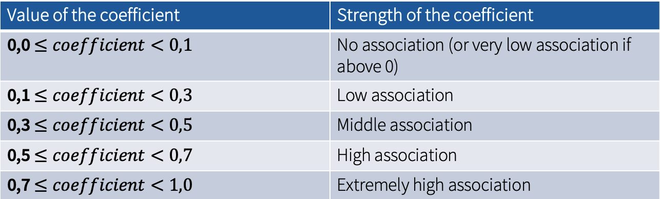
cramers_v

The resulting values should be: Phi (φ) = 0.460368442189626; Cramer‘s V = 0.4603684. Based on Kuckartz et al. (2013), these values correspond to a middle-sized association between the variables.

5.4 Correlation

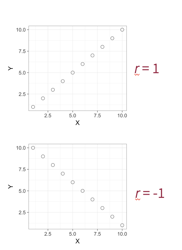
Correlation is an undirected linear relationship between two metric variables. Since we always look at the relationship between two variables, this is referred to as a bivariate relationship.

The primary question correlation addresses is: Is there a connection between two variables?

Two variables are linearly related if they vary linearly with each other, also known as covariation. This linear relationship can manifest in two different ways:

• Positive correlation = High (low) values of one variable are associated with high (low) values of the second variable.

  • For example:

    • The more a person eats, the more pronounced is their sense of satiety.

    • The less a person eats, the lower their feeling of satiety.

• Negative correlation = High (low) values of one variable are associated with low (high) values of the other variable.

  • For example:

    • The more a person sleeps, the less tired he is.

    • The less a person sleeps, the more tired he is.

The correlation coefficient ranges from -1 (perfect negative correlation) to 1 (perfect positive correlation).

Rule of thumb:

• r = +/- 0.10 weak correlation

• r = +/- 0.30 moderate correlation

• r = +/- 0.50 strong correlation

Apart from the correlation coefficient, we are also interested in the p-value → p < .05 = significant

5.4.1 Correlation in R

The contact hypothesis (Allport, 1954) assumes that contact with members of an “outgroup” (based on nationality, religion, etc.) can reduce prejudice. Using the dataset Prejudice_Refugees (largely representative sample, N = 765), we can see see whether there’s really a correlation.

Research question: Is there a connection between contact with refugees (Contact_Refugees) and prejudices against refugees (Prejudices_Refugees)?

There are multiple correlation coefficients as well as many possible ways of calculating them in R:

• Pearson’s r (linear relationships, moderate and large samples, continuous variables)

• Spearman’s rho (monotonic relationships, small samples, ordinal or continuous variables)

• Kendall’s tau (small samples, only ordinal variables)

  

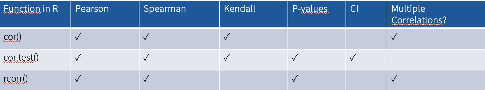
→ in this course we will use Pearson’s R

First, we need to load the dataset Prejudice_Refugeesto R:

prejudice_refugees <- read_sav("Prejudice_Refugees.sav")

Next, we want to use the function rcorr() from package Hmisc to get the correlation coefficient. However, this function works only with matrices. Therefore, we need to transform our data into a matrix first:

correlation_matrix <- as.matrix(prejudice_refugees[, c("Prejudice_refugees", 
"Contact_refugees")])

Now we need to install and load the Hmisc package:

install.packages("Hmisc")
library(Hmisc)

Then we can apply the rcorr() function on the newly created matrix:

rcorr(correlation_matrix)

The result will look like this:

> rcorr(correlation_matrix)
                   Prejudice_refugees Contact_refugees
Prejudice_refugees               1.00             0.08
Contact_refugees                 0.08             1.00

n= 765 


P
                   Prejudice_refugees Contact_refugees
Prejudice_refugees                    0.026           
Contact_refugees   0.026   

We can see that the correlation coefficient (Pearson’s R) is 0.08, which is a weak positive correlation. This relationship is significant as p = 0.026, i.e, p < .05 =>Contact with refugees was significantly related to prejudice towards refugees.

5.4.2 Partial correlation

The fact that two variables are correlated does not mean there is a causal relationship between them. There can be other variables at play, causing the two variables to appear to be related to each other. To exclude the influence of third-party variables, their effects must be controlled in a model. This can be done using various statistical methods, such as partial correlation or multiple regression.

Partial correlation checks whether there is a linear relationship between two variables, taking into account the effects of one or more additional variables (control variables).

5.4.2.1 Partial correlation in R

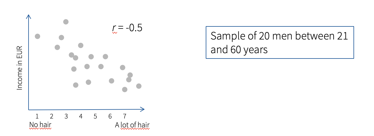
Hypothesis: Men with bald heads are richer than men with hair. In this case, age is a possible influencing variable, without controlling for age, a false correlation can occur.

To control for age, we can use the function pcor from ppcor package to calculate partial correlation.

First, we need to load the dataset to R:

hair <- read_sav("Hair.sav")

Then, we need to install and load the ppcor package:

install.packages("ppcor")
library(ppcor) 

Now we can run the partial correlation:

pcor(hair[, c("Hair", "Income", "Age")])

The result will look like this:

$estimate
             Hair    Income        Age
Hair    1.0000000 0.1353157 -0.6378657
Income  0.1353157 1.0000000  0.7086814
Age    -0.6378657 0.7086814  1.0000000

$p.value
              Hair       Income          Age
Hair   0.000000000 0.5807182674 0.0032995269
Income 0.580718267 0.0000000000 0.0006825949
Age    0.003299527 0.0006825949 0.0000000000

$statistic
             Hair    Income       Age
Hair    0.0000000 0.5631002 -3.414914
Income  0.5631002 0.0000000  4.141530
Age    -3.4149137 4.1415303  0.000000

$n
[1] 20

$gp
[1] 1

$method
[1] "pearson" 

We can see that when we control for age, the correlation between amount of hair and income is no longer significant (r= 0.135, p = 0.581).

5.5 Participation Exercise 5

The fifth participation exercises includes 3 smaller exercises

5.5.0.1 Participation Exercise 5.1. Step-by-step instructions

1. Open the STADA project (STADA.RProj) and create a new R Script
2. Load the package haven
3. Install and load package gmodels
4. Load the dataset Gender_behavior.sav to R, using the read_sav function:

gender_behavior <- read_sav("Gender_behavior.sav")

5. Use the following code snippet to do the Chi-square analysis to find out whether there’s a relationship between gender and introversion/extraversion. Do not forget to plug in the name of the dataset (gender_behavior) and the variables (Gender and Introvert_Extrovert):

CrossTable(datasetname$variable1, datasetname$variable2,
chisq = TRUE, fisher = TRUE, expected = TRUE, sresid = TRUE, format = "SPSS")

6. Copy paste the output (or make a screenshot) to a Word file and interpret the results.

5.5.0.2 Participation Exercise 5.2. Step-by-step instructions

1. Install and load package Hmisc

2. Load the dataset Prejudice_Refugees.sav to R, using the read_sav function

3. We are interested whether positive experiences with refugees (Negative_experiences_refugees) correlate with prejudice towards refugees (Prejudice_refugees). First, we need to transform our data into matrix. Use the following code snippet and do not forget to plug in the name of the dataset and the variables:

correlation_matrix <- as.matrix(datasetname[, c("variable1", "variable2")])

4. Now run calculate the Pearson’s R correlation coefficient and p-value using the rcorr function:

rcorr(correlation_matrix)

5. Copy paste the output (or make a screenshot) to a Word file and interpret the results.

5.5.0.3 Participation Exercise 5.3. Step-by-step instructions

1. Now we want to find out whether political ideology (Ideology) plays a role in this relationship.

2. Install and load package ppcor

3. Run a partial correlation model using the function pcor. Plug into the following code snippet names of the dataset and variables:

pcor(datasetname[, c("variable1", "variable2", "variable3")])

4. Copy paste the output (or make a screenshot) to a Word file and interpret the results.

5. Save the RScipt as PE5_lastname.R. Save the Word file as a pdf, name it PE5_lastname.pdf and upload both on Moodle.