11 Confidence intervals

In the last chapter, we discussed sampling distributions of estimators, and in this chapter, we use sampling distributions to construct confidence intervals for population parameters. This is one of the most used ways to perform statistical inference on parameters of interest.

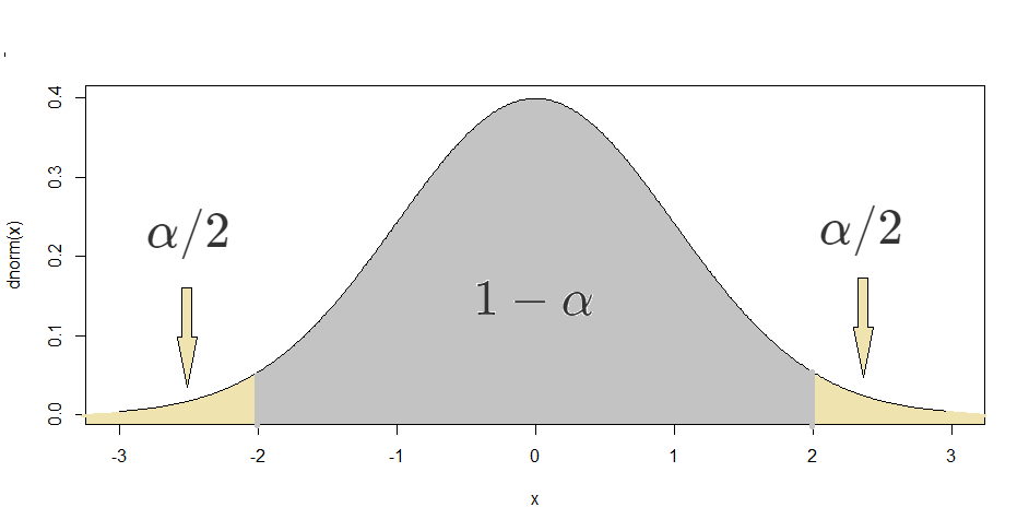
In sections 2.6 and 5.1, we have mentioned a threshhold of 0.05 for p-values when performing hypothesis tests. This cutoff value is reffered to as the significance level of a test and is usually denoted by \(\alpha\). For confidence intervals, we use a confidence level instead of a significance level, which is usually \(1-\alpha\). For example, \(\alpha = 0.05\) implies a confidence level of \(0.95\) (95%).

Definition 11.1 A \((1-\alpha)\) confidence interval (CI) for a population parameter \(\theta\) is a random interval \([L, U]\) such that \([L, U]\) includes \(\theta\) with probability \(1-\alpha\). That is, \(P(L\leq \theta \leq U)=1-\alpha.\)

We call the interval \([L,U]\) random for the same reason we call estimators random variables; different samples will produce different intervals. For example, if a 95% confidence interval for \(\mu\) is \([8.1, 9.4]\), this means that the probability that \(\mu\) is within \([8.1, 9.4]\) is 0.95. The population parameter is a fixed number, not a random variable, but because confidence intervals are random intervals, sometimes they will not capture the population parameter and that’s why we need to quantify our confidence that we captured it.

In what follows, we develop ways of constructing confidence intervals for common population parameters of interest.

11.1 Confidence interval for \(\mu\)

The goal in this subsetion is to construct a \((1-\alpha)\) confidence interval for the population mean \(\mu\), using a random sample of the population.

Theorem 11.1 (Confidence interval for one mean) Consider an iid sample \(X_1, X_2, \dots, X_n\) with \(E(X_i) = \mu\) and \(Var(X_i) = \sigma^2\). Then the endpoints of a \((1-\alpha)\) CI for \(\mu\) are given by \[ \overline{X}\pm c\times \frac{S}{\sqrt{n}}, \quad \mbox{where } c = qnorm(1-\alpha/2). \] That is, the \((1-\alpha)\) CI is: \[ \left[\overline{X} - c\times \frac{S}{\sqrt{n}}, \overline{X} + c\times \frac{S}{\sqrt{n}}\right], \quad \mbox{where } c = qnorm(1-\alpha/2). \]

Proof. For large enough \(n\) (usually \(n\geq 30\) suffices), the Central Limit Theorem says that \(\frac{\overline{X}-\mu}{\sigma/\sqrt{n}} \approx N(0,1).\) We can begin the construction of the confidence interval by using the symmetry of the normal PDF to find \(c\) such that \(P(-c\leq \frac{\overline{X}-\mu}{\sigma/\sqrt{n}}\leq c) = 1-\alpha.\) This is equivalent to finding \(c\) such that \(P(\frac{\overline{X}-\mu}{\sigma/\sqrt{n}} \leq c) = 1-\alpha/2\) (see figure below with the \(N(0,1)\) PDF.) Therefore, \(c\) is the inverse CDF of the standard normal distribution evaluated at \(1-\alpha/2.\) Using R’s notation, this is \(qnorm(1-\alpha/2).\) Notice that we omit the values 0 and 1 in the input of qnorm. This is because in the absence of the parameters of the normal distribution, R uses the standard normal parameters, 0 and 1. Finally, with some algebra, one can show that the statement \[P\left(-c\leq \frac{\overline{X}-\mu}{\sigma/\sqrt{n}}\leq c\right) = 1-\alpha\] is equivalent to \[P\left(\overline{X}-c\frac{\sigma}{\sqrt{n}} \leq \mu \leq \overline{X}+c\frac{\sigma}{\sqrt{n}}\right) = 1-\alpha.\] In practice, we usually don’t have access to \(\sigma\), so we use the estimator \(S\) in its place. For large enough \(n\), this substitution is appropriate and yields reliable confidence intervals.

{width = 0.7} `

Example 11.1 Suppose that we would like to

The following is a version of theorem 11.1 when the \(X_i\)’s take only the values 0 and 1.

Theorem 11.2 (Confidence interval for one proportion) Consider an iid sample \(X_1, X_2, \dots, X_n\) of 0s and 1s with \(E(X_i) = p\) and \(Var(X_i) = p(1-p)\). Then the endpoints of a \((1-\alpha)\) CI for \(p\) are given by \[ \hat{p}\pm c\times \sqrt{\frac{\hat{p}(1-\hat{p})}{n}}}, \quad \mbox{where } c = qnorm(1-\alpha/2). \] That is, the \((1-\alpha)\) CI is: \[ \left[\overline{X} - c\times \sqrt{\frac{\hat{p}(1-\hat{p})}{n}}}, \overline{X} + c\times \sqrt{\frac{\hat{p}(1-\hat{p})}{n}}}\right], \quad \mbox{where } c = qnorm(1-\alpha/2). \]

Example 11.2