1.9 The mean and standard deviation
The mean and standard deviation (SD) are the most common ways to summarize the center and spread of a distribution. Here are the key points that you should know for this class. These points are explained further in the text below.
Key points about the mean and SD
To summarize the typical value of a unimodal, symmetric distribution, use the mean
To summarize the variability of a unimodal, symmetric distribution, use the standard deviation
The range of likely results in a unimodal, symmetric distribution are those that are within 2 SD of the mean
1.9.1 Mean
In this class, we’ll generally use the mean to describe the center of a distribution, or the “typical” value in a distribution. Many people think of the mean in terms of how it is calculated: add up all of the values in a distribution, and divide by the number of data points. But that doesn’t really tell us much. You might wonder, what kind of center does this give us? Why should this give us a summary of the “typical” value? To answer these questions, consider the football kick activity. Recall, that in the football kick activity, we used the mean as our “best guess” for where a given kick was going to land.
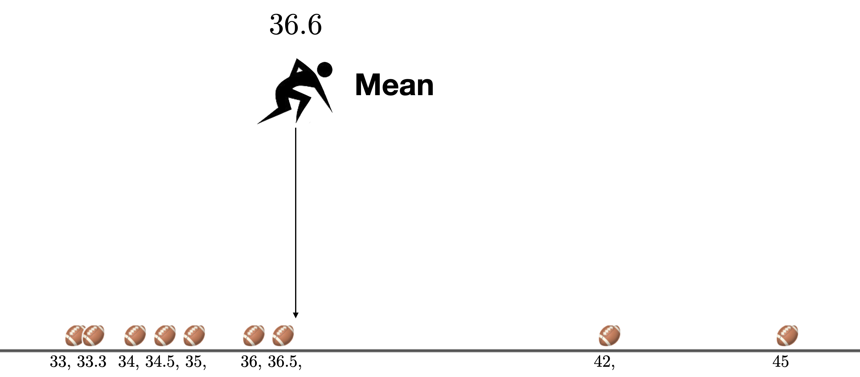
Figure 1.5: The mean is the “best guess” for where a given kick will land.
At first, it may seem strange to think about the mean as the “best guess” for where the next ball is going to land.
For one, the mean, 36.6 yards, is not even one of the existing distances. If the judge knew the mean in advance and had been standing there the entire time, none of the balls would have landed there! That doesn’t seem like a great guess.
For two, there are more kicks below the mean than there are kicks above the mean. If the judge had been standing at the mean for the entire time, she would have had to run backwards (left in our picture) more times than she would have had to forwards.
And yet, in this course and in most statistical practice, the mean is the most common measure of “center.” In mathematical theory the “Expected value” of a random variable (that is, the “best guess” for where the next kick is going to land) is defined as the long-run mean of the data.
So just what kind of “center” does the mean give us?
If the judge had been standing at the mean for each kick, she would have had to run to the left 7 times and to the right 2 times. To understand the mean, instead of counting how many times she ran to the left or right, we focus on the total distance that she ran to the left and to the right.
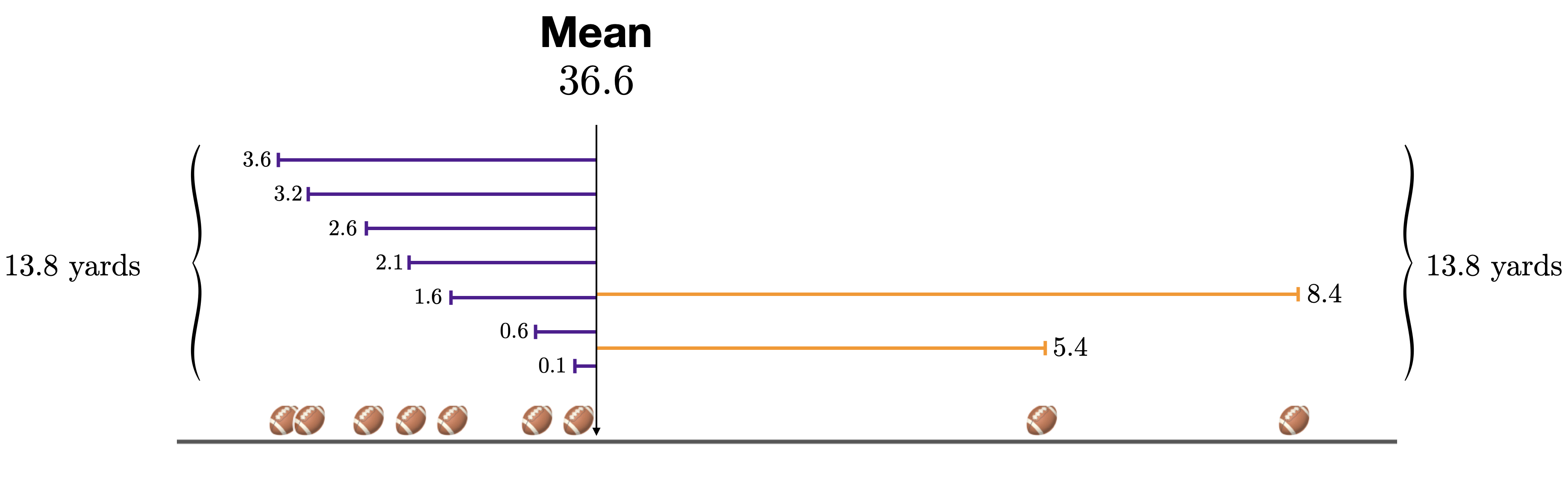
Figure 1.6: The mean is the precise point that balances the deviations.
Then we can see that the mean is the precise point where the deviations to the left are exactly equal to the deviations to the right. It does not systematically under-estimate or over-estimate, and this is why it is a good way to describe the “typical” value in a distribution.
Some useful ways to think of the mean are:
The mean:
- The mean is a summary of the center or typical value in a distribution.
- The mean equalizes the deviations. It does not systematically under-estimate or over-estimate.
- The mean is the balance point of the distribution. If you put a dot plot of the distribution on a see-saw, the mean is the point where it would be balanced
- The mean is the break-even point. If you were to bet on the mean, in the long run you will lose exactly as much money as you will win.
- The mean is the fair share. If you made very data point equal, they would all equal the mean.
1.9.2 Standard deviation (SD)
The standard deviation is the most common way to measure the variability in a distribution. Variability is at the heart of statistics, as Franklin et al. (2005)10 explain:
Statistical thinking, in large part, must deal with the omnipresence of variability; statistical problem solving and decision making depend on understanding, explaining, and quantifying the variability in the data. It is this focus on variability in data that sets apart statistics from mathematics.
To understand the standard deviation, and how it measures variability, let’s return to the football kick activity.
If we lived in a perfectly mathematical world, every kicker would be perfectly precise, and we wouldn’t need to use statistical reasoning to help the judge to know where to stand. The judge would know exactly where to stand, and every single kick would land there. There would be no variability:

Figure 1.7: A world with no variability. Every kick lands in the exact same place.
But we don’t live in a mathematical world, we live in a statistical world, where there is some variability associated with every kicker.
Of course, not every kicker has the same variability. Some kickers have more variability than others.
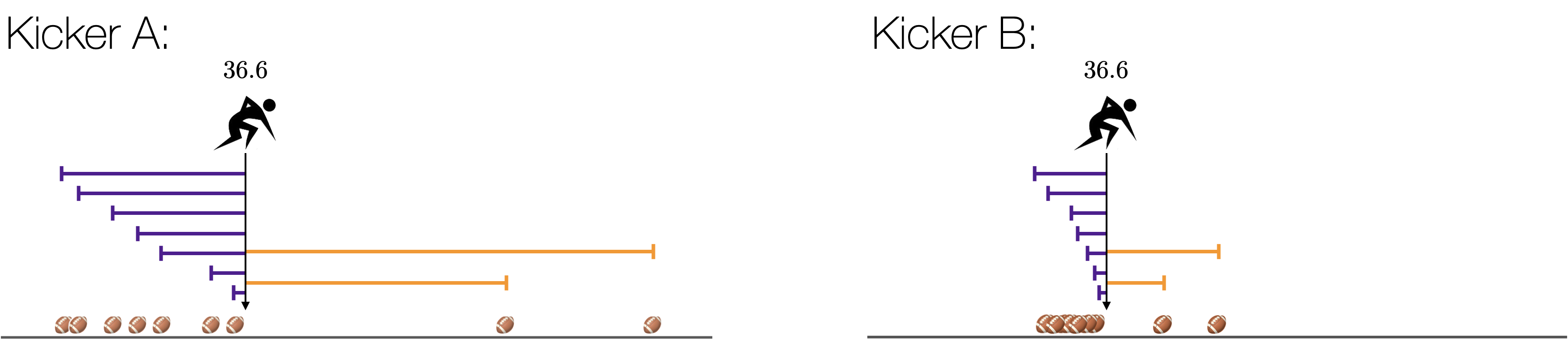
Figure 1.8: Two kickers.
In the figures above, both kickers have a mean (an expected value) of 36.6. However, Kicker A has more variability than Kicker B. But how much more variable is Kicker A? We would like to be able to quantify the variability.
One way to think about variability in the football kicks is to the think about how far the judge expects to run on a given kick. If the kicker has a lot of variability, the kicks will be spread out away from the mean and the judge will expect to run far each time. If the kicker has very little variability, the kicks will be clustered close to the mean and the judge will expect to run less.
In statistics, we call each of the arrows a “deviation” from the mean. When the distribution has a lot of variability, the deviations tend to be large (Kicker A). When the distribution has little variability, the deviations tend to be small (Kicker B).
We can quantify the variability in a distribution by summarizing the size of a “typical” deviation—that is, how far the judge expects to run on a given kick. This is (basically) what the standard deviation does. If the word “typical” is substituted for the word “standard” in its name, the name standard deviation (typical deviation) makes more sense. This measure quantifies variability by determining how far data cases typically deviate from the mean.11
⏯ You can learn more about the standard deviation by watching this video.
Some useful ways to think about the standard deviation are:
The standard deviation (SD):
- The SD is a measure of spread or variation in a distribution.
- The SD is tells us the typical deviation of a data point from the mean.
- When the SD is large, the data tend to be spread out from the mean. When the SD is small, the data points tend to be clustered close to the mean.
1.9.3 Range of likely results
In a unimodal, symmetric, “bell-shaped” distribution, the heart of the distribution is within 1 SD of the mean:
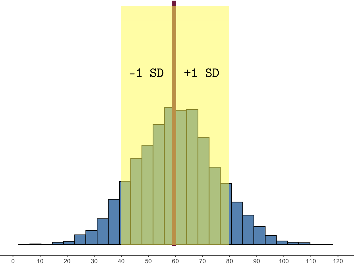
Figure 1.9: The heart of the distribution is within 1 SD of the mean.
And about 95% of the data fall within 2SD of the mean:
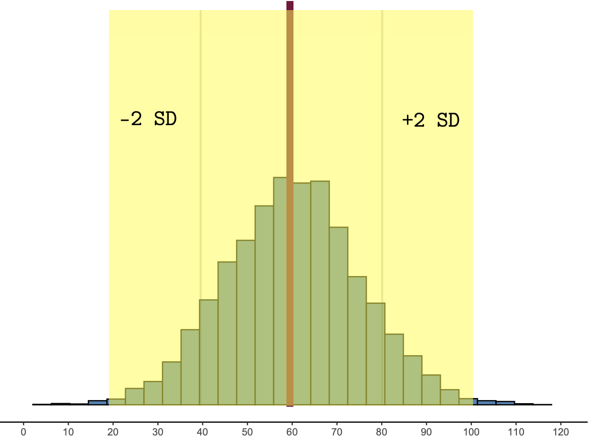
Figure 1.10: About 95% of the data are within 2 SD of the mean.
Most statisticians define likely results as those that are within two standard deviations of the mean. Anything more than two standard deviations from the mean would be called unlikely.
Range of likley results:
The range of likely results are those that are within two standard deviations of the mean. Anything more than two standard deviations from the mean would be called unlikely.
Franklin, C. A., Kader, G. D., Mewborn, D. S., Moreno, J., Peck, R., Perry, M., & Scheaffer, R. L. (2005). Guidelines for assessment and instruction in statistics education (GAISE) report: A pre-k–12 curriculum framework. https://doi.org/10.3928/01484834-20140325-01↩︎
The details of how to calculate the standard deviation are a bit complex. We won’t ever calculate a standard deviation by hand in this class. However, if you’d like to know how to do it, you can watch this video↩︎