2 Statistique descriptive
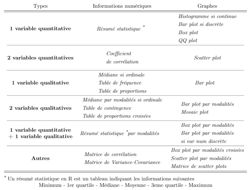
Que faut-il faire pour décrire numériquement et / ou visualiser tel type de variable?
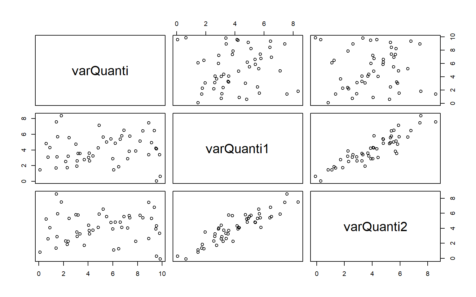
Afin d’illuster certaines fonctions nous allons utiliser le jeu de données suivant:
set.seed(123)
cat1 <- c(rep("H",25), rep("F",25))
cat2 <- c(rep("Grp1",17), rep("Grp2",17), rep("Grp3",16))
Quanti1 = rnorm(50,4,2)
df <- data.frame(varQuanti = runif(50,0,10),
                 varQuanti1 = Quanti1,
                 varQuanti2= Quanti1+rnorm(50,0,1),
                 varQuali = sample(cat1, replace=TRUE),
                 varQuali1 = sample(cat1, replace=TRUE),
                 varQuali2 = sample(cat2, replace=TRUE))
# On extrait uniquement les variables quantitatives de df
df_quanti <- subset(df, select=c(varQuanti, varQuanti1, varQuanti2))
Ce sont des données fictives, inventées de toute pièce. Il y a 3 variables quantitatives: varQuanti varQuanti1 varQuanti2 ainsi que 3 variables qualitatives varQuali varQuali2 varQuali3. Ces données se trouvent dans un dataframe nommé df et les 3 variables quantitatives uniquement dans df_quanti.
2.1 Numérique
2.1.1 Tendance centrale
- Moyenne ~>
mean() - Médiane ~>
median()
2.1.2 Variabilité
- Minimum / maximum ~>
min()/max() - Range ~>
range() - Variance ~>
var() - Ecart-type ~>
sd() - Covariance ~>
cov()
2.1.3 Quantiles
- Quantile ~>
quantile()
- Ecarte interquartile ~>
IQR()
2.1.4 Autres
- Résumé statistique ~>
summary()
| Min. | 1st Qu. | Median | Mean | 3rd Qu. | Max. |
|---|---|---|---|---|---|
| 0.1047 | 2.596 | 5.049 | 5.154 | 7.358 | 9.842 |
- Table de fréquence ou contingence ~>
table() - Table de proportion ~>
prop.table()
| F | H |
|---|---|
| 22 | 28 |
| Grp1 | Grp2 | Grp3 | |
|---|---|---|---|
| F | 2 | 9 | 10 |
| H | 8 | 10 | 11 |
- Table de proportion ~>
prop.table()
| F | H |
|---|---|
| 0.44 | 0.56 |
- Coefficient / matrice de corrélation ~>
cor()
| varQuanti | varQuanti1 | varQuanti2 | |
|---|---|---|---|
| varQuanti | 1 | 0.06801 | 0.02392 |
| varQuanti1 | 0.06801 | 1 | 0.9014 |
| varQuanti2 | 0.02392 | 0.9014 | 1 |
- Matrice de Variance-Covariance ~>
cov()
| varQuanti | varQuanti1 | varQuanti2 | |
|---|---|---|---|
| varQuanti | 8.645 | 0.3703 | 0.1364 |
| varQuanti1 | 0.3703 | 3.429 | 3.237 |
| varQuanti2 | 0.1364 | 3.237 | 3.761 |
- Informations par modalités ~>
tapply()
res <- tapply(df$varQuanti, df$varQuali, FUN = summary) # summary de df$varQuanti par modalité de df$varQualiF:
Min. 1st Qu. Median Mean 3rd Qu. Max. 0.6072 2.226 3.606 4.564 7.358 9.353 H:
Min. 1st Qu. Median Mean 3rd Qu. Max. 0.1047 3.603 5.746 5.617 7.63 9.842
2.2 Graphique
2.2.3 Histogramme ~> hist()
hist(df$varQuanti, freq = TRUE ,
     main = "Histogramme d'une variable uniforme",
     xlab = "Variable quantitative uniforme")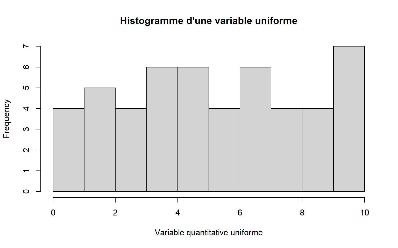
2.2.4 Bar plot ~> barplot()
# Une variable qualitative
barplot(table(df$varQuali2), main = "Bar plot d'une variable qualitative")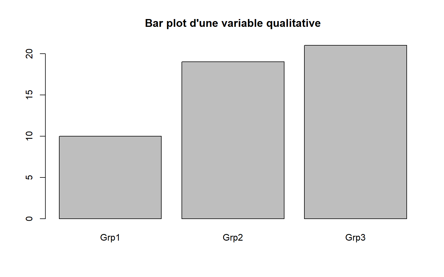
# 2 variables qualitatives
barplot(table(df$varQuali1,df$varQuali2), beside = TRUE, legend = levels(df$varQuali1),
        main ="Barplot par modalités")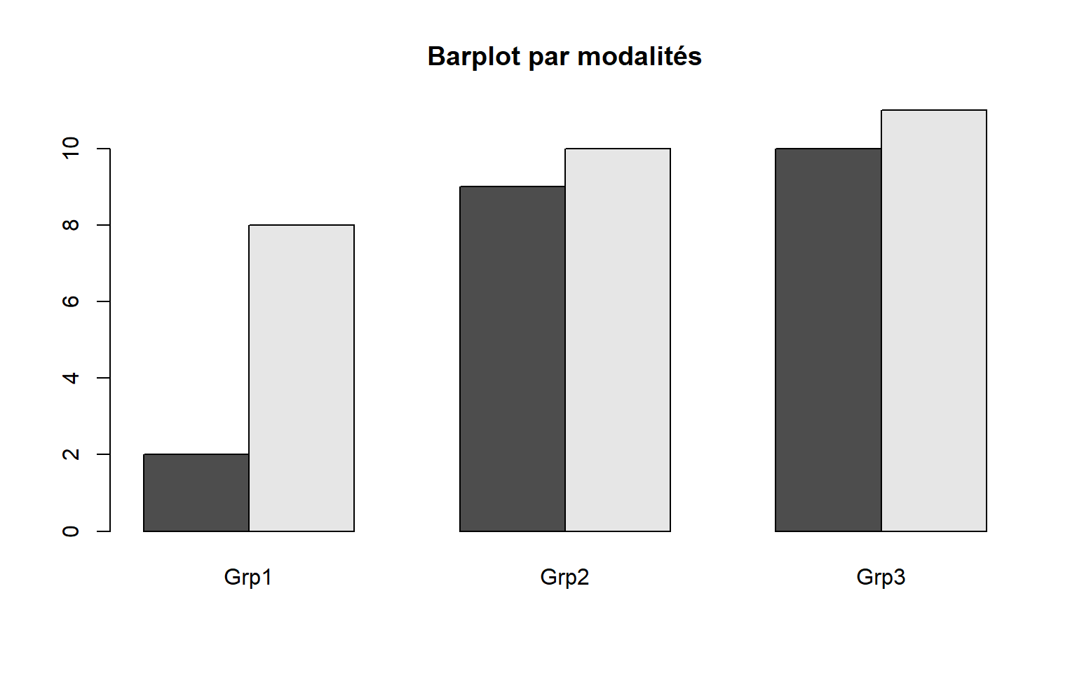
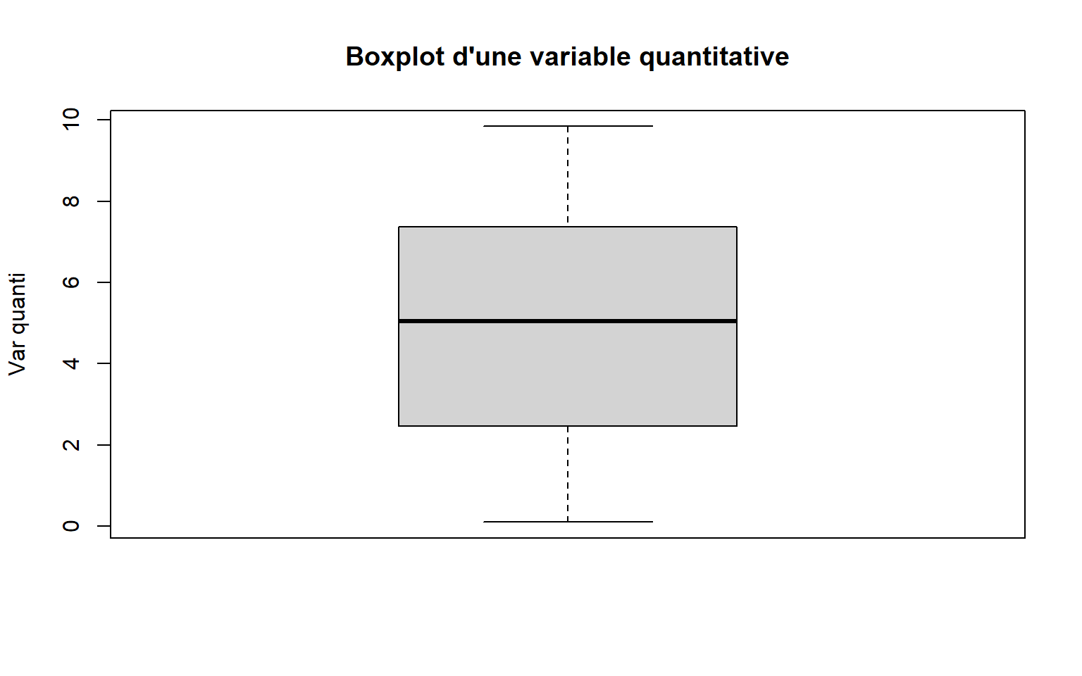
2.2.5 Box plot ~> boxplot()
# Par modalités
boxplot(varQuanti ~ varQuali, data = df,
        main = "Boxplot d'une variable quantitative par modalités",  ylab = "Var quanti")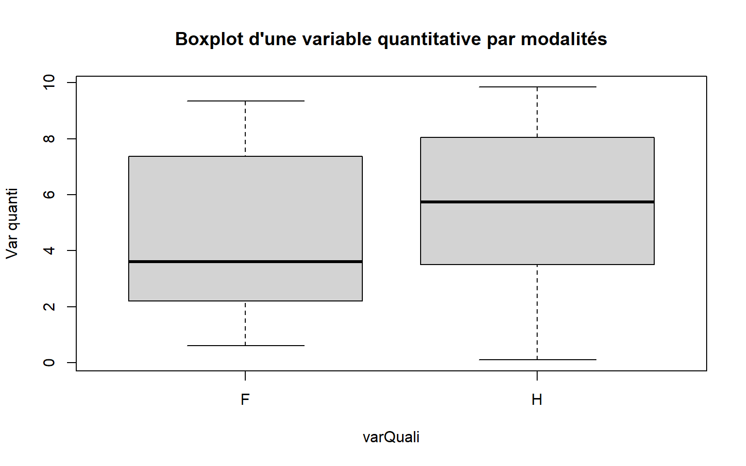
# Par modalités croisées
boxplot(varQuanti ~ varQuali1*varQuali2, data = df,
        main = "Boxplot d'une variable quanti par modalités croisées",  ylab = "Var quanti")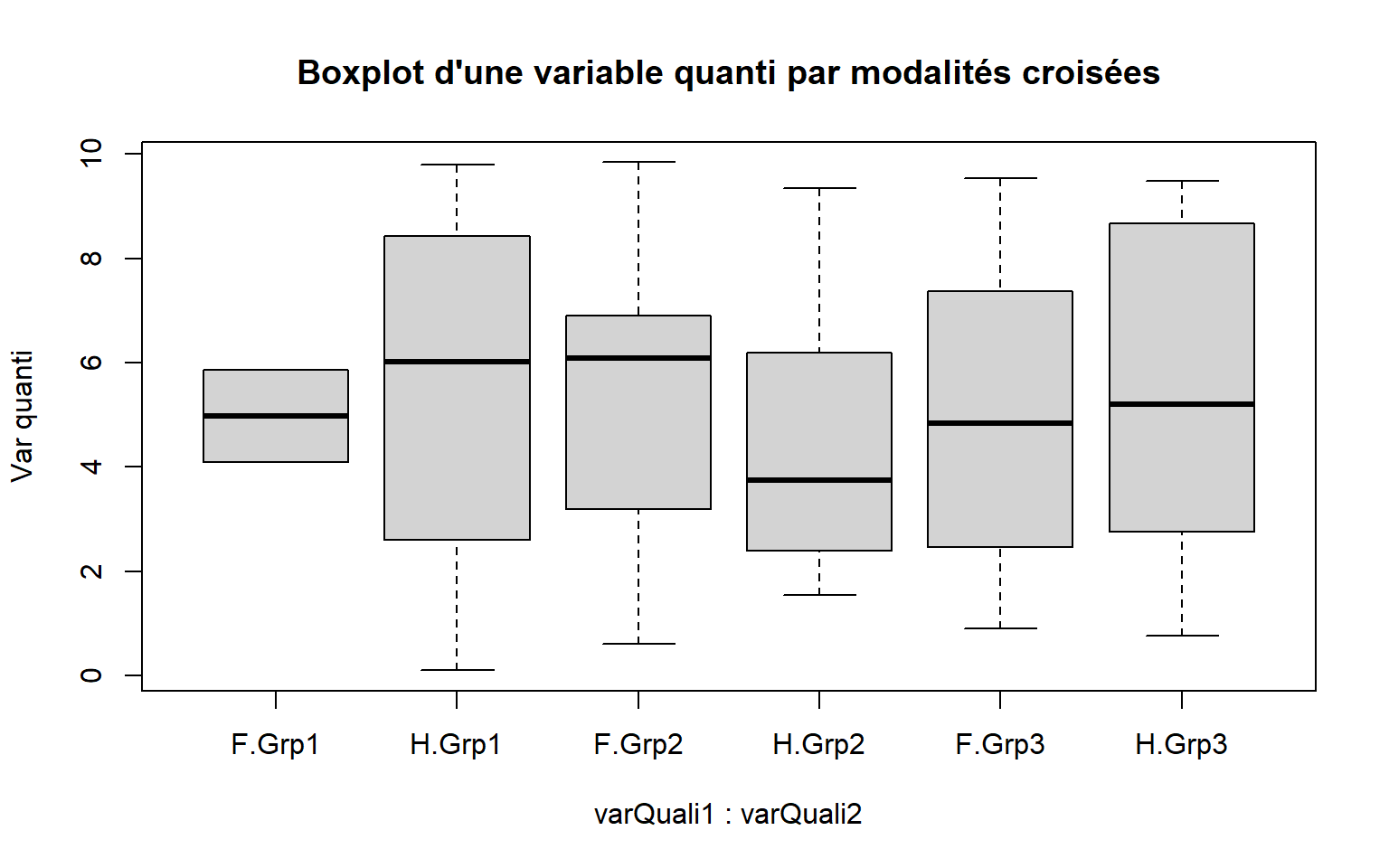
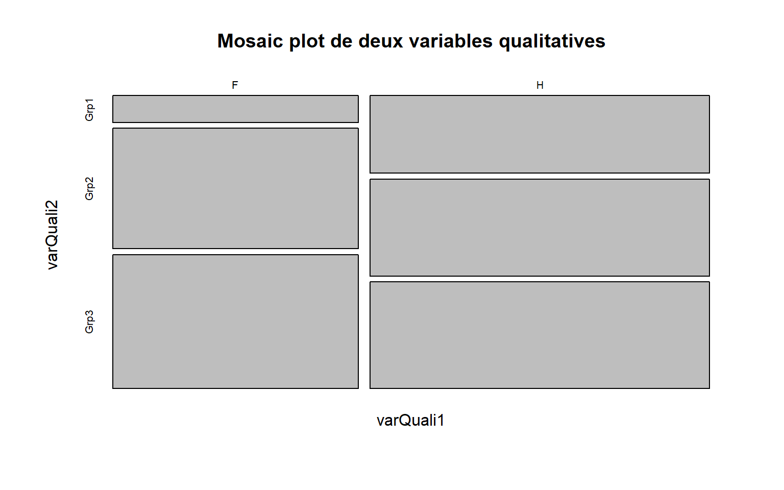
2.2.6 Mosaic plot ~> mosaicplot()
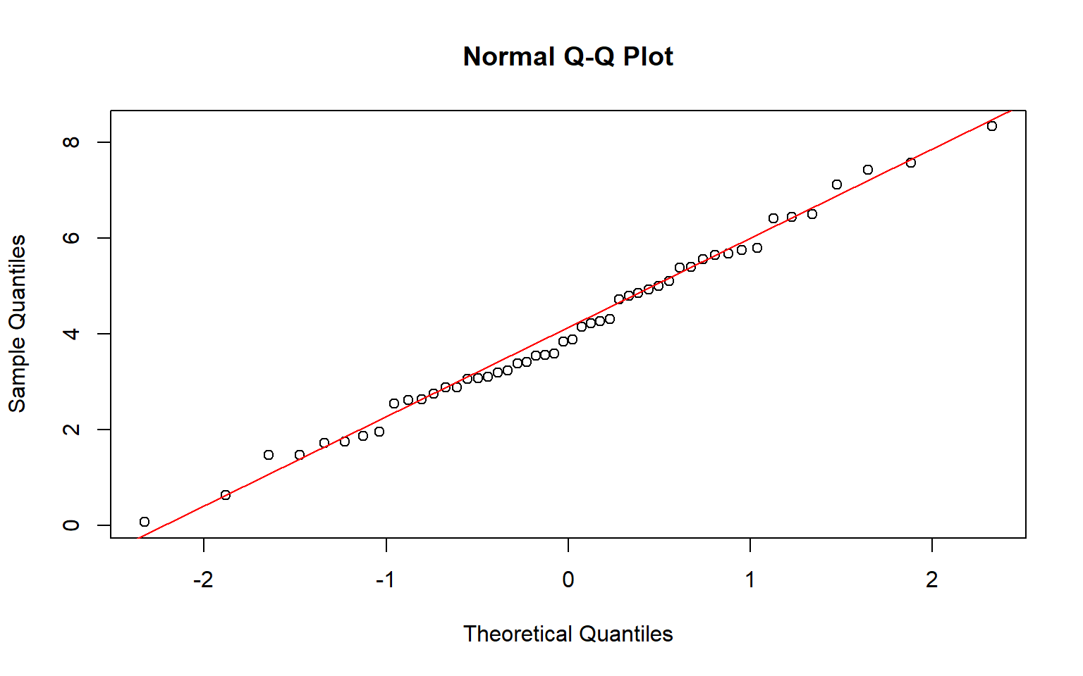
2.2.7 QQ-plot ~> qqnorm() + qqlines()