Module 5B Generalized Additive Models

Motivation and Examples

Motivation

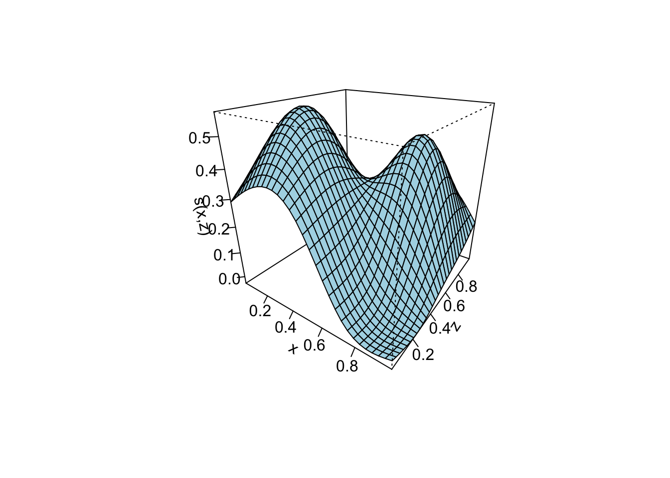
Module 5A focused on additive nonlinear effects, \[ g(\mathbb{E}[Y]) = \beta_0 + \sum_{j=1}^p s_j(X_j), \] which assumes that each predictor \(j\) has its own smooth effect, but those smooth functions do not interact or vary by group. This rules out two common features of real data:

(1) Smooth Interactions: the effect of \(X\) may change smoothly across levels of another variable \(Z\). In other words, the shape of a smooth function \(s(X)\) depends on \(Z\), meaning the joint effect is a smooth surface rather than two separate additive curves.

(2) Group-specific smooth functions and clustering: Smooth functions may differ by group (effect modification across individuals, regions, clinics, etc.). These situations introduce clustering that cannot be handled by a simply additive GAM. They require either (a) varying-coefficient smooths (smooths allowed to differ by group), or (b) explcit random effects.

Goal of Module 5B: add (1) smooth interactions via tensor products; (2) varying-coefficient smooths.

---

Two-Dimensional Smooth Interactions via Tensor-Product Smooths

First, consider the setting where we have two continuous predictors, \(x\) and \(z\), and the outcome \(y\) depends on them in a jointly nonlinear way. In this situation, modeling the effect of \(x\) and the effect of \(z\) separately is not enough; instead, we need a smooth bivariate surface \(s_{12}(x,z)\) that captures how the effect of one variable changes smoothly across levels of the other.

This scenario arises in many applications. For example:

• the joint effect of temperature and humidity on asthma ER visits,
• how altitude and latitude together influence plant growth,
• the combined influence of age and blood pressure on cardiovascular risk,
• or the joint relationship between longitude and latitude in spatial smoothing.

In all of these settings, the two variables interact in a way that cannot be represented by a single univariate smooth, nor by smoothing the product \(xz\). Instead, we need a flexible framework for estimating a smooth surface over the \((x,z)\) plane.

Tensor-product smooths provide exactly this framework. They are built by combining the univariate spline bases for \(x\) and \(z\) and then penalizing curvature separately in each direction.

The next section explains how these smooth surfaces are constructed using spline bases and anisotropic penalties.

Model

For two continuous predictors \(x\) and \(z\), the model is given by \[ g(\mathbb{E}[Y]) = \beta_0 + s_1(x) + s_2(z) + s_{12}(x,z), \] where

1. \(s_1(x)\): a smooth effect of \(x\).
2. \(s_2(z)\): a smooth effect of \(z\), and
3. \(s_{12}(x,z)\) a smooth interaction between \(x\) and \(z\).

\(s_{12}(x,z)\) is not a smooth of the product \((xz)\). Instead it is a bivariate smooth function- a flexible surface over the 2D plane formed by \((x,z)\).

Bivariate smoothing example

Basis and Penalty

To construct a smooth surface \(s_{12}(x,z)\), we begin with the same building blocks used in univariate GAMs: basis functions and smoothness penalties. A tensor-product smooth represents a bivariate surface by combining the marginal spline bases for \(x\) and \(z\).

1. Basis Construction

Let

• \(\mathbf{b}_x(x) \in \mathbb{R}^{Q}\) be the spline basis for \(x\), and
  
• \(\mathbf{b}_z(z) \in \mathbb{R}^{P}\) be the spline basis for \(z\).

For example, these could be cubic B-splines.

A tensor-product smooth constructs a bivariate basis by pairing every basis function in \(x\) with every basis function in \(z\). This is achieved using the row-wise Kronecker product:

\[ \mathbf{b}_{xz}(x,z) = \mathbf{b}_x(x) \otimes \mathbf{b}_z(z), \]

• \(b_x(x) = (b_{x1}(x), b_{x2}(x), …, b_{xQ}(x)))^T\)
• \(b_z(z) = (b_{z1}(z), b_{z2}(z), …, b_{zP}(z)))^T\) Each is simply the univariate basis you learned in 5A.

What Is a Kronecker Product?

Tensor–product smooths rely on a mathematical operation called the Kronecker product, denoted by \(\otimes\). The Kronecker product combines two matrices to form a larger matrix with a clear block structure, and it provides the machinery for building bivariate spline bases from two univariate bases.

Definition

If \[ A \text{ is } m \times n, \qquad B \text{ is } p \times q, \] then the Kronecker product \(A \otimes B\) is an \((mp) \times (nq)\) matrix obtained by multiplying every element of \(A\) by the entire matrix \(B\).

Formally,

\[ A \otimes B = \begin{pmatrix} a_{11} B & a_{12} B & \cdots & a_{1n} B \\ a_{21} B & a_{22} B & \cdots & a_{2n} B \\ \vdots & \vdots & \ddots & \vdots \\ a_{m1} B & a_{m2} B & \cdots & a_{mn} B \end{pmatrix}. \]

Example

Let

\[ A = \begin{pmatrix} a & b \\ c & d \end{pmatrix}, \qquad B = \begin{pmatrix} 1 & 2 \\ 3 & 4 \end{pmatrix}. \]

Then

\[ A \otimes B = \begin{pmatrix} aB & bB \\ cB & dB \end{pmatrix} = \begin{pmatrix} a & 2a & b & 2b \\ 3a & 4a & 3b & 4b \\ c & 2c & d & 2d \\ 3c & 4c & 3d & 4d \end{pmatrix}. \]

Each entry of \(A\) becomes a block equal to that entry multiplied by the whole matrix \(B\).

Using this construction, the smooth surface is:

\[ s_{12}(x,z) = \mathbf{b}_{xz}(x,z)^\top \boldsymbol{\beta}. \]

• \(\mathbf{b}_{xz}(x,z)\) is the vector of basis functions evaluated at \((x,z)\) of length \(Q\cdot P\).
• \(\mathbf{\beta}\) is the corresponding vector of spline coefficients also length \(Q\cdot P\).
• This allows the effect of \(x\) to vary smoothly across values of \(z\), and vice versa.

2. Penalty Construction

From Module 5A, we learned about penalties for curvature:

\[ \text{Penalty} = \lambda \int [s''(x)]^2 \, dx \]

where \(s''(x)\) is the second derivative (curvature).
The smoothing parameter \(\lambda\) controls wiggliness: larger \(\lambda\) values produce smoother functions.

For a spline written as \(s(x) = \mathbf{b}_x(x)^\top \boldsymbol{\beta}\), the curvature penalty becomes

\[ \text{Penalty} = \lambda\, \boldsymbol{\beta}^\top \mathbf{K} \boldsymbol{\beta}. \]

Here:

• \(\boldsymbol{\beta}\) = spline coefficients
  
• \(\lambda\) = smoothing parameter
  
• \(\mathbf{K}\) = penalty matrix representing the integral of squared curvature

Extending to bivariate smooths

In one dimension, each smooth has its own penalty matrix. For the marginal smooths:

• \(\mathbf{K}_x\) controls curvature in the \(x\)-direction (a \(Q \times Q\) matrix)
  
• \(\mathbf{K}_z\) controls curvature in the \(z\)-direction (a \(P \times P\) matrix)

For a bivariate smooth, we now have a grid of \(Q \times P\) tensor-product basis functions. To smooth the full surface, we must extend the 1D penalties across this grid.

The idea is:

• the \(x\)-penalty should apply to every \(z\)-basis function
  
• the \(z\)-penalty should apply to every \(x\)-basis function

This extension is achieved using Kronecker products with identity matrices.

Interpreting the Tensor-Product Penalty

The full penalty for a bivariate tensor-product smooth is

\[ \mathcal{P}(\boldsymbol{\beta}) = \lambda_x\, \boldsymbol{\beta}^\top (\mathbf{K}_x \otimes \mathbf{I}_{P})\, \boldsymbol{\beta} \;+\; \lambda_z\, \boldsymbol{\beta}^\top (\mathbf{I}_{Q} \otimes \mathbf{K}_z)\, \boldsymbol{\beta}. \]

Below we break this expression into two interpretable pieces—one for the \(x\)-direction and one for the \(z\)-direction.

1. \(x\)-direction smoothing term

\[ \lambda_x\, \boldsymbol{\beta}^\top (\mathbf{K}_x \otimes \mathbf{I}_{P})\, \boldsymbol{\beta}. \]

Components:

• \(\mathbf{K}_x\)
  The univariate curvature penalty matrix for the \(x\)-basis functions
  (size \(Q \times Q\)).

• \(\mathbf{I}_{P}\)
  Identity matrix of size \(P \times P\), one for each \(z\)-basis function.

• \(\mathbf{K}_x \otimes \mathbf{I}_P\)
  Kronecker product that repeats \(\mathbf{K}_x\) across all \(P\) columns of the \(Q \times P\) tensor-product grid.
  This applies the \(x\)-direction curvature penalty to every \(z\)-basis function.

• \(\lambda_x\)
  Smoothing parameter controlling how much we penalize wiggliness in the \(x\)-direction.

Interpretation:
This term smooths the surface horizontally. It controls how wiggly the surface can be if we vary \(x\) while holding \(z\) fixed.

2. \(z\)-direction smoothing term

\[ \lambda_z\, \boldsymbol{\beta}^\top (\mathbf{I}_{Q} \otimes \mathbf{K}_z)\, \boldsymbol{\beta}. \]

Components:

• \(\mathbf{K}_z\)
  The univariate curvature penalty matrix for the \(z\)-basis functions
  (size \(P \times P\)).

• \(\mathbf{I}_{Q}\)
  Identity matrix of size \(Q \times Q\), one for each \(x\)-basis function.

• \(\mathbf{I}_Q \otimes \mathbf{K}_z\)
  Kronecker product that repeats \(\mathbf{K}_z\) down all \(Q\) rows of the tensor-product grid.
  This applies the \(z\)-direction curvature penalty to every \(x\)-basis function.

• \(\lambda_z\)
  Smoothing parameter controlling how much we penalize wiggliness in the \(z\)-direction.

Interpretation:
This term smooths the surface vertically. It controls how wiggly the surface can be if we vary \(z\) while holding \(x\) fixed.

A tensor-product smooth is a \(Q \times P\) grid of basis functions.
To make the resulting surface smooth:

• \(\mathbf{K}_x \otimes \mathbf{I}_P\)
  smooths along the \(x\)-direction (left–right across the grid)

• \(\mathbf{I}_Q \otimes \mathbf{K}_z\)
  smooths along the \(z\)-direction (up–down across the grid)

Together, these two terms allow the model to control smoothness separately in each direction—important when \(x\) and \(z\) are measured on very different scales or units.

---

Fitting Example in R

Coming back to the example in Module 5A, we are interested in the association between daily variation in mortality counts and daily variation in air pollution exposure (PM\(_{2.5}\)). In a time-series design, the population serves as the unit of analysis—our outcome represents total daily deaths in a defined area.

As before, time-varying confounders such as temperature, humidity, and long-term/seasonal trends must be controlled flexibly using smooth functions of time and weather. In this dataset, we have:

• alldeaths: total daily deaths
  
• pm25: daily PM\(_{2.5}\) (or pm25.lag1 for lagged exposure)
  
• Temp: daily mean temperature
  
• DpTemp: daily mean dew point temperature (a proxy for humidity)
  
• date2: numeric time index
  
• fdow: day-of-week factor

We model the expected daily deaths using a log–link Poisson GAM:

\[ \begin{aligned} \log \mathbb{E}[y_t] &= \beta_0 \;+\; f_{\text{Temp,PM}}\!\big(\text{Temp}_t,\, \text{PM}_{t-1}\big) \;+\; \boldsymbol{\alpha}^\top \mathbf{1}\{\text{DOW}_t\} \\[4pt] &\quad+\; f_{\text{Season}}(\text{DOY}_t) \;+\; f_{\text{Trend}}(t), \end{aligned} \]

where:

• \(y_t\) is the daily death count (e.g., alldeaths),
  
• \(\text{Temp}_t\) is the daily mean temperature,
  
• \(\text{PM}_{t-1}\) is lagged PM\(_{2.5}\) (e.g., pm25.lag1),
  
• \(\mathbf{1}\{\text{DOW}_t\}\) are indicators for day-of-week,
  
• \(f_{\text{Season}}(\text{DOY}_t)\) is a cyclic seasonal smooth (e.g., s(doy, bs = "cc")),
  
• \(f_{\text{Trend}}(t)\) is a smooth long-term trend in time (e.g., s(date2)).

The bivariate smooth interaction is represented as

\[ f_{\text{Temp,PM2.5}}(x, z) = \sum_{q=1}^{Q} \sum_{p=1}^{P} \beta_{qp}\, b_{xq}(x)\, b_{zp}(z), \]

where

• \(\{b_{xq}(x)\}_{q=1}^{Q}\) are the basis functions for temperature,
  
• \(\{b_{zp}(z)\}_{p=1}^{P}\) are the basis functions for PM\(_{2.5}\),
  
• \(\beta_{qp}\) are the coefficients for the tensor-product basis functions \(b_{xq}(x) b_{zp}(z)\).

Smoothness in each direction is controlled separately via anisotropic penalties:

\[ \lambda_x\, \boldsymbol{\beta}^\top (\mathbf{K}_x \otimes \mathbf{I}_{P})\, \boldsymbol{\beta} \;+\; \lambda_z\, \boldsymbol{\beta}^\top (\mathbf{I}_{Q} \otimes \mathbf{K}_z)\, \boldsymbol{\beta}, \]

library(mgcv)

load(paste0(getwd(), '/data/NYC.RData'))
health$date2 <- order(health$date)
health$pm25.lag1 <- c(NA, health$pm25[1:1825])
health$doy <- as.integer(format(health$date, "%j"))   # Day of year
health$fdow <- factor(health$dow)
health$fdow <- relevel(health$fdow, ref = "Sunday")


mod_tensor <- gam(
  alldeaths ~ 
    te(Temp, pm25.lag1) + # smooth interaction: temperature × air pollution. Deafult k=10
    s(doy, bs = "cc", k = 30) + # cyclic annual seasonality
    s(date2, k = 100) + # long-term trend
    fdow,        # day-of-week
  family = poisson,
  data   = health
)

summary(mod_tensor)

Family: poisson 
Link function: log 

Formula:
alldeaths ~ te(Temp, pm25.lag1) + s(doy, bs = "cc", k = 30) + 
    s(date2, k = 100) + fdow

Parametric coefficients:
              Estimate Std. Error z value Pr(>|z|)    
(Intercept)   4.952756   0.005220 948.832  < 2e-16 ***
fdowFriday    0.009615   0.007355   1.307   0.1911    
fdowMonday    0.033186   0.007314   4.538 5.69e-06 ***
fdowSaturday  0.003926   0.007360   0.533   0.5938    
fdowThursday  0.013130   0.007352   1.786   0.0741 .  
fdowTuesday   0.016740   0.007340   2.281   0.0226 *  
fdowWednesday 0.014038   0.007349   1.910   0.0561 .  
---
Signif. codes:  0 '***' 0.001 '**' 0.01 '*' 0.05 '.' 0.1 ' ' 1

Approximate significance of smooth terms:
                      edf Ref.df Chi.sq  p-value    
te(Temp,pm25.lag1)  5.135  6.091   63.6  < 2e-16 ***
s(doy)             16.684 28.000   22.0 2.79e-06 ***
s(date2)           58.397 68.874  371.2  < 2e-16 ***
---
Signif. codes:  0 '***' 0.001 '**' 0.01 '*' 0.05 '.' 0.1 ' ' 1

R-sq.(adj) =   0.48   Deviance explained = 50.2%
UBRE = 0.12532  Scale est. = 1         n = 1825

Interpretation:

The tensor‐product smooth for Temp × pm25.lag1 is statistically significant \((p < 2e−16)\), indicating that the joint effect of temperature and lagged PM\(_{2.5}\) on daily mortality is not simply additive. Certain combinations of higher PM\(_{2.5}\) and temperature are associated with elevated mortality risk, consistent with known temperature-pollution interactions. You can inspect the marginal basis dimensions via:

mod_tensor$smooth[[1]]$margin[[1]]$bs.dim   # basis size for Temp

[1] 5

mod_tensor$smooth[[1]]$margin[[2]]$bs.dim   # basis size for pm25.lag1

[1] 5

The maximum dimension of the tensor-product basis in \(Q \times P = 5 \times 5 = 25\), but the penalty shrinks many directions towards zero. Because the smooth is penalized, only a subset of these directions are used in the final fit. Inspecting the \(EDF \approx 5.1\), this means after penalization, the estimated surface behaves like a smooth with roughly 5 free parameters.

Note: In the univariate case (s(x)), the default basis size is \(k = 10\). This is not the default for tensor-product smooths. For te(x, z), mgcv does not automatically use \(k = 10\) for each marginal smooth. Instead, it typically assigns smaller default basis sizes (often \(k = 5\) for each margin) unless the user specifies k = c(k_x, k_z) explicitly.

---

Varying-Coefficient Smooths (Effect Modification)

Tensor-product smooths allow a fully flexible two-dimensional surface when two continuous predictors jointly influence the outcome. However, many applied problems require a different—but related—form of flexibility: the effect of a predictor may change across groups, but not in a fully two-dimensional continuous way.

Examples include:

• the temperature–mortality curve differing by season,
  
• the PM\(_{2.5}\) effect varying by weekday vs. weekend,
  
• growth curves differing by sex,
  
• time trends differing by site, clinic, or neighborhood.

In these settings we are not modeling a smooth surface over the continuous \((x,z)\) plane. Instead, we want the univariate smooth \(s(x)\) to vary by group in a structured and parsimonious way. This is called a varying-coefficient smooth.

---

Motivation

Suppose we believe the effect of PM\(_{2.5}\) on mortality differs between weekdays and weekends. A single smooth \(s(\text{PM})\) cannot represent two different shapes. Instead, we allow:

\[ s_{\text{weekday}}(\text{PM}) \quad\text{and}\quad s_{\text{weekend}}(\text{PM}). \]

But we should not fit two unrelated smooths. Instead, we build them as:

• a baseline smooth \(s(\text{PM})\), plus
  
• a difference smooth that captures how weekends deviate from weekdays.

This preserves identifiability and allows the two curves to share information.

---

Model

Let \(G\) be a binary or categorical grouping variable.
A varying-coefficient smooth model is:

\[ g(\mathbb{E}[Y]) = \beta_0 + \beta_G G + s(x) + s(x,\text{by}=G). \]

Interpretation:

• \(s(x)\) = baseline smooth, common to all groups
  
• \(s(x,\text{by}=G)\) = group-specific difference curves
  
• \(\beta_G G\) = parametric main effect (required for identifiability)

This is the smooth analogue of an interaction between \(x\) and \(G\).

---

Basis Representation

Mathematically, a varying-coefficient smooth expands the basis functions across groups. Let \(G\) have \(C\) categories and let \(b_m(x)\) be the \(k\) basis functions for \(s(x)\). Then

\[ s(x) + s(x,\text{by}=G) = \sum_{m=1}^k \beta_m\, b_m(x) \;+\; \sum_{c=1}^{C-1} \sum_{m=1}^k \gamma_{mc}\, b_m(x)\, I(G=c), \]

where \(I(G=c)\) is the group indicator. The first term is the baseline smooth (for the reference group). The second term contains \((C-1)\) group-specific deviation smooths, each using the same basis functions but different coefficients. Adding the baseline and deviation smooths yields a complete smooth for every group.

---

Group-specific penalties

Each smooth term in a varying–coefficient model receives its own smoothing penalty. If \(G\) has \(C\) categories, then s(x) has one penalty \(\lambda_{\text{base}}\), and the \((C-1)\) deviation smooths s(x, by = G) have their own penalties $,* , `. Thus the full penalty is

\[ \lambda_{\text{base}}\,\boldsymbol{\beta}^\top K \boldsymbol{\beta} \;+\; \sum_{c=1}^{C-1} \lambda_c\,\boldsymbol{\gamma}_c^\top K \boldsymbol{\gamma}_c. \] Each group (except the reference) has its own deviation smooth:

• \(\boldsymbol{\gamma}_c\)
  Coefficient vector for the deviation smooth of group \(c\).
  This describes how group \(c\)’s smooth curve differs from the baseline smooth.

• Same penalty matrix \(K\)
  The deviation smooths use the same spline basis as the baseline,so the same curvature penalty applies.

• \(\boldsymbol{\gamma}_c^\top K \boldsymbol{\gamma}_c\)
  Measures how wiggly the deviation curve is for group \(c\).

• \(\lambda_c\)
  Smoothing parameter for the deviation smooth of group \(c\).
  Large \(\lambda_c\) shrinks the deviation toward zero (group curve becomes similar to the baseline).
  Small \(\lambda_c\) allows a flexible, group-specific shape.

---

Example: PM2.5 Effect Varies by Day-of-Week

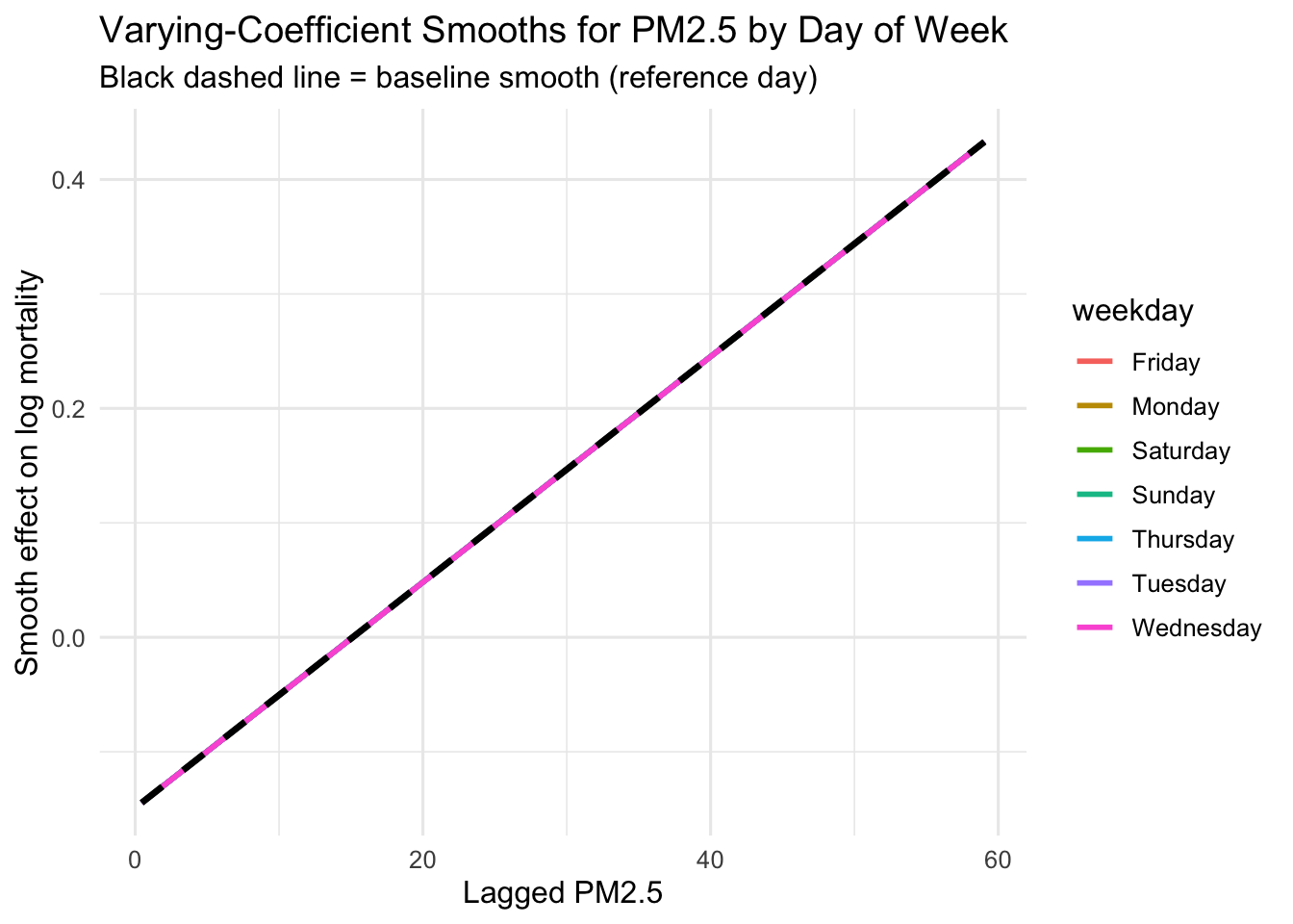
Using the NYC mortality data, suppose we want the PM\(_{2.5}\)–mortality relationship to differ across days of the week.

mod_vc <- gam(
  alldeaths ~ 
    s(pm25.lag1) +# baseline smooth
    s(pm25.lag1, by = fdow) + # day-of-week differences
    s(doy, bs = "cc", k = 30) +
    s(date2, k = 100),
  family = poisson,
  data = health
)

summary(mod_vc)

Family: poisson 
Link function: log 

Formula:
alldeaths ~ s(pm25.lag1) + s(pm25.lag1, by = fdow) + s(doy, bs = "cc", 
    k = 30) + s(date2, k = 100)

Parametric coefficients:
            Estimate Std. Error z value Pr(>|z|)    
(Intercept) 4.966015   0.001974    2516   <2e-16 ***
---
Signif. codes:  0 '***' 0.001 '**' 0.01 '*' 0.05 '.' 0.1 ' ' 1

Approximate significance of smooth terms:
                              edf Ref.df  Chi.sq p-value    
s(pm25.lag1)                1.000  1.000   1.544   0.214    
s(pm25.lag1):fdowSunday     3.664  4.717   7.035   0.292    
s(pm25.lag1):fdowFriday     4.445  5.422   8.916   0.142    
s(pm25.lag1):fdowMonday     1.000  1.000   1.183   0.277    
s(pm25.lag1):fdowSaturday   1.000  1.000   1.237   0.266    
s(pm25.lag1):fdowThursday   1.000  1.001   1.254   0.263    
s(pm25.lag1):fdowTuesday    1.719  2.171   1.793   0.398    
s(pm25.lag1):fdowWednesday  1.000  1.000   1.413   0.235    
s(doy)                     17.981 28.000  27.149  <2e-16 ***
s(date2)                   54.108 64.497 343.777  <2e-16 ***
---
Signif. codes:  0 '***' 0.001 '**' 0.01 '*' 0.05 '.' 0.1 ' ' 1

Rank: 199/200
R-sq.(adj) =  0.465   Deviance explained = 48.7%
UBRE = 0.15709  Scale est. = 1         n = 1825

Interpretation

PM\(_{2.5}\) effects

• The baseline smooth s(pm25.lag1) has edf = 1.0, meaning the smooth pooled across all days of the week is effectively linear.

• All group-specific deviation smooths (s(pm25.lag1, by = fdowX)) have very low EDFs (mostly 1–2) and are not statistically significant.

• There is no evidence that the PM\(_{2.5}\)–mortality relationship is nonlinear and no evidence that this relationship varies by day of week.

• PM\(_{2.5}\) appears to have a consistent linear effect across weekdays.

Seasonality and long-term trend

• s(doy) (day-of-year) has edf ≈ 18, p < 2e−16 → strong seasonal mortality pattern.
• s(date2) has edf ≈ 54, p < 2e−16 → substantial smooth long-term trend over the study period.

Conclusion

• Adding varying-coefficient smooths does not materially improve fit.
• Weekday-specific PM\(_{2.5}\) effects are weak or absent in this dataset.
• Seasonal and long-term trends remain the dominant smooth components.

---

Summary

Topic	Summary
What is new?	Module 5B extends Module 5A by introducing: (1) tensor-product smooths for smooth interactions between two continuous variables, producing a bivariate surface \(s_{12}(x,z)\); and (2) varying-coefficient smooths using by= to allow the effect of a predictor to differ across categorical groups.
Tensor-product basis	A bivariate smooth is constructed from the tensor (Kronecker) product of the marginal spline bases. If \(\mathbf{b}_x(x)\in\mathbb{R}^Q\) and \(\mathbf{b}_z(z)\in\mathbb{R}^P\), then the surface basis is:
Anisotropic penalties	Smoothness in each direction is controlled separately. Let \(\mathbf{K}_x\) and \(\mathbf{K}_z\) be the marginal curvature penalty matrices. The tensor-product penalty is:
Varying-coefficient smooths	When the effect of a predictor varies by group, the model uses a baseline smooth plus group-specific deviation smooths:
Penalties for varying-coefficient terms	Each smooth receives its own curvature penalty:
Estimation	All smoothing parameters—\(\lambda_x,\lambda_z\), the baseline smooth penalty, and group-specific penalties—are estimated using REML (preferred) or GCV. Penalization controls smooth complexity and prevents overfitting.
Uncertainty	mgcv provides approximate Bayesian covariance for spline coefficients, yielding pointwise confidence bands for univariate smooths and uncertainty surfaces for tensor-product smooths.
Diagnostics	Use gam.check() to assess whether the basis dimension \(k\) is adequate. Inspect EDF to understand smooth complexity. Use concurvity() to detect nonlinear dependencies across smooth terms.
Interpretation	Tensor-product interactions are interpreted via 2D heatmaps or 3D perspective surfaces of \(s_{12}(x,z)\). Varying-coefficient models are interpreted by comparing the baseline smooth and group-specific deviation curves. Interpretations occur on the link scale.
Key takeaway	GAMs allow effects to be nonlinear, interactive, and group-specific, while penalization maintains interpretability. Tensor-product smooths model flexible 2D surfaces; varying-coefficient smooths model structured effect modification—greatly extending the GAM framework introduced in Module 5A.