Using \(gam()\) in package \(mgcv()\) to fit semiparametric models with parametric slopes and nonparametric terms.
Bivariate splines
Interpreting non-linear effects
Motivation and Examples
Motivation
In Module 4 we learned about basis expansions and parametric splines. These introduce smooth functions to capture non-linear relationships between outcome and covariates. We saw examples where:
The outcome is Gaussian.
There is one non-linear covariate
How can we extend this to multivariable and non-normal settings while keeping models interpretable and smoothness data-driven?
Answer: Generalized Additive Model: A GAM models the mean via a link: \[
g\!\big(\mathbb{E}[Y]\big) = \beta_0 + \sum_{j=1}^p s_j(X_j),
\] where \(g(\cdot)\) is the link, \(s_j(\cdot)\) are smooth functions (e.g., splines), and \(p\) is the number of predictors.
where:
\(Y\) is the response variable,
\(g()\) is the link function that relates the expected value of \(Y\)\((E(Y)\) to the linear predictor.
\(\beta_0\) is the intercept term.
\(s_j(X_j)\) are smooth functions, such as splines, applied to the predictor variable \(X_j\).
\(p\) is the number of predictor variables.
Each smooth function \(s_j(\cdot)\) allows for greater flexibile, non-linear relationships between \(Y\) and \(X_j\).
Why GAMs?
Flexible: captures separate nonlinear effects \(s_j(X_j)\) for each predictor.
Interpretable: additive structure → clear partial effects and plots.
Automatic smoothing: each \(\lambda\) is learned from the data (e.g., REML/GCV).
Extensible: include factors, linear terms, and interactions via tensor-product smooths (e.g., \(s_{12}(x_1,x_2)\)).
Motivating Example: Low Birthweight in GA Recall from example in Module 3.
Dataset: a cohort of live births from GA born in the year 2001 (N=77,340)
Variables:
\(ptb\): indicator for preterm birth for whether baby from pregnancy \(i\) was born <37 weeks.
\(age\): mothers age at delivery
\(male\): indicator of baby’s sex (1=male, 0=female)
\(tobacco\): indicator for mother tobacco use during pregnancy test (1=yes, 0=no)
In previous analysis, we fit this using a logistic regression model, which assumed a Bernoulli data model with a logit-link. We regressed the outcome (probability of low-birth weight) on age, sex, and tobacco status.
But we may want to account for non-linear age effect:
Note: By default, mgcv::gam() uses cubic regression splines (bs = "cr") with k = 10 basis functions (including the intercept of the smooth).
library (mgcv)library(ggplot2)library(dplyr)# Pre-term births with non-linear age effectload(paste0(getwd(), '/data/PTB.RData'))fit.gam =gam(ptb~s(age) + male + tobacco ,family = binomial, data = dat)summary(fit.gam)
The response variable ptb is modeled using a binomial family with a logit link function.
The formula includes:
A smooth term for age (s(age)).
Linear terms for male and tobacco.
Intercept: The log-odds of ptb when all predictors are at their reference levels is estimated as \(-2.44\) (highly significant, \(p < 2 \times 10^{-16}\)).
maleM (male effect): Being male is associated with a small but significant increase in the log-odds of ptb (estimate = \(0.073\), \(p = 0.00494\)). Tobacco use is associated with a significant increase in the log-odds of ptb (estimate = \(0.39\), \(p < 3.24 \times 10^{-13}\)).
Smooth Term for Age (s(age)) : The smooth function for age has an estimated effective degrees of freedom (edf) of \(3.31\), indicating a moderately flexible relationship. Is highly significant (\(p < 2 \times 10^{-16}\)), suggesting a non-linear relationship between age and the log-odds of ptb.
Adjusted\(R^2\): The model explains only \(0.177\%\) of the variability in the response, indicating weak predictive power.
Deviance explained: The model accounts for \(0.304\%\) of the total deviance, further supporting limited explanatory capability. -
UBRE score: - A measure of model fit, with a value of \(-0.42095\). UBRE is similar to AIC for non-normal data: Lower is better!
Sample size: - The model was fit on \(77,340\) observations.
Conclusion: While the predictors (age, male, and tobacco) show significant associations with ptb, the overall model has limited explanatory power for predicting ptb.
Checking GAMs
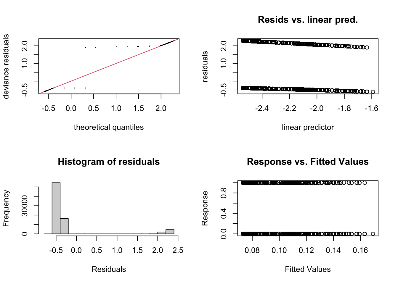
mgcv::gam.check(fit.gam)
Method: UBRE   Optimizer: outer newton
full convergence after 3 iterations.
Gradient range [9.816712e-07,9.816712e-07]
(score -0.4209495 & scale 1).
Hessian positive definite, eigenvalue range [1.285937e-05,1.285937e-05].
Model rank =  12 / 12

Basis dimension (k) checking results. Low p-value (k-index<1) may
indicate that k is too low, especially if edf is close to k'.

         k'  edf k-index p-value
s(age) 9.00 3.31    0.95    0.72
Interpretation:
Residual plots for fitted values are a good way to check residuals in the normal case. But for binary outcomes, they look odd and are not helpful.
\(k' = 9\rightarrow\) the smooth for age was represented using 9 basis functions (default).
\(edf=3.31\rightarrow\) the effective degrees of freedom are much lower than 9, indicating that the smooth for age is relatively simple- not over wiggly or overfitted. It if is close to \(k\) then it is overfitting.
\(k-index = 0.94\) and \(p-value = 0.44 \rightarrow\)
No evidence that the basis dimension \(k\) is too small.
The smooth has enough flexibility to capture the nonlinear pattern in age.
If the k-index were close to 0 or p-value < 0.05, it would suggest that the smooth is constrained by too few basis functions and should be increased.
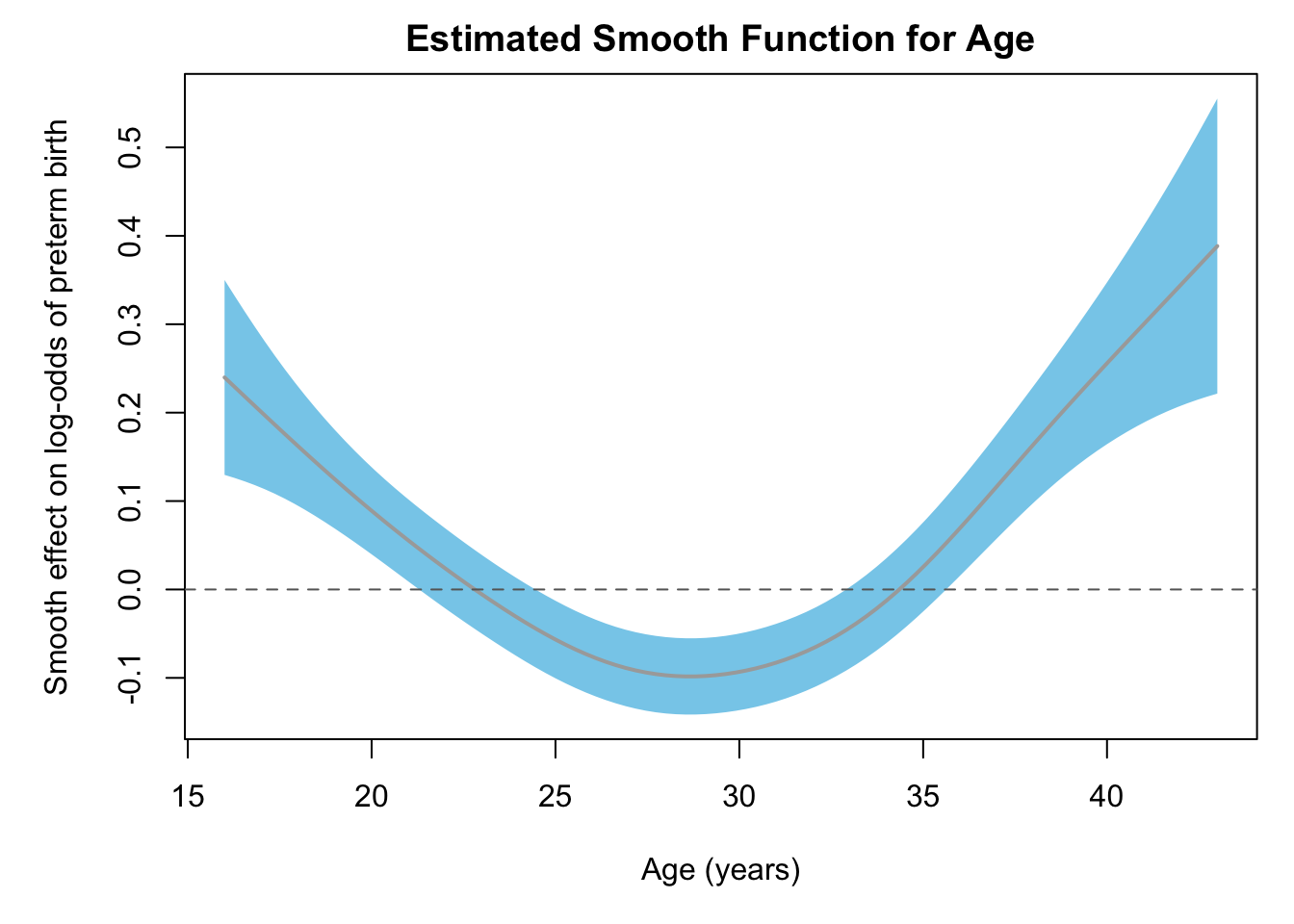
Looking at the plot below, what is the trend of age and preterm birth?
Biologically, log-odds of preterm birth is higher at very young ages, lowest around 29 years, and then increased again.
Multiple Smoothers
So far, we have focused on fitting a single smooth function. In real-world applications, we often have multiple predictors, each contributing its own nonlinear effect on the response. This leads to additive models with multiple smooth components.
Consider the model with two continuous variables \(x_i\) and \(z_i\):
\(g_1(\cdot)\) and \(g_2(\cdot)\) are smooth, potentially nonlinear functions of their respective predictors.
The model can be extended to generalized responses (e.g., binomial, Poisson) through an appropriate link function.
Each smooth can be written as a basis expansion with a curvature penalty: \[
\begin{aligned}
g_1(x) &= \sum_{m=1}^{M_1} \beta_{m1}\, b_{m1}^{(d)}(x),\qquad
g_2(z) = \sum_{m=1}^{M_2} \beta_{m2}\, b_{m2}^{(d)}(z),
\end{aligned}
\] with roughness penalties
where \(\ell(\boldsymbol{\beta}\mid \mathbf{y})\) is the log-likelihood for the chosen GLM family (e.g., binomial, Poisson, quasi-Poisson).
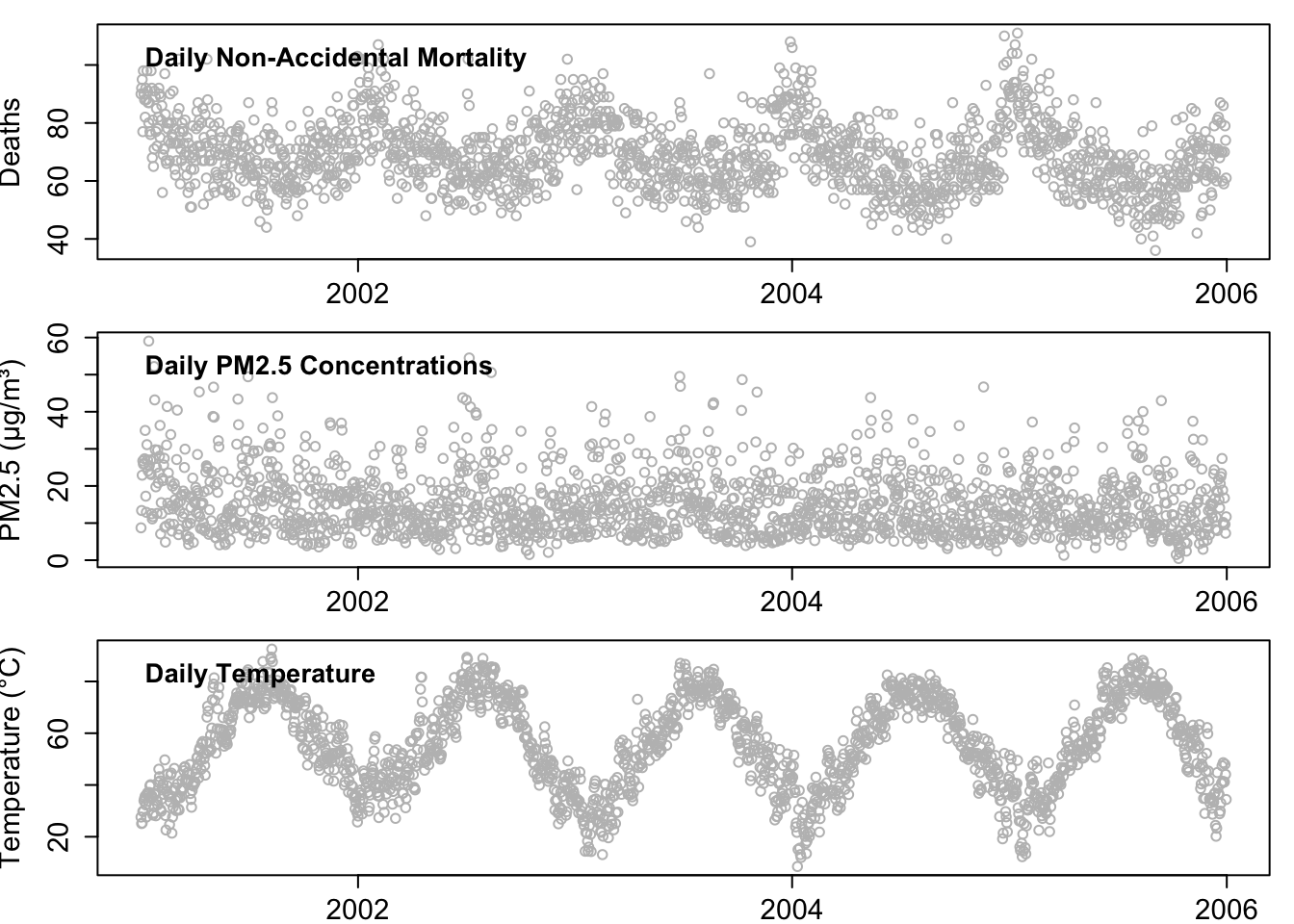
Motivating Example: Air Pollution and Mortality
Scientific Question: What is the association between daily mortality counts and daily concentrations of fine particulate matter (PM₂.₅)?
Context:
Fine particulate matter (PM₂.₅) consists of solid and liquid particles in the air with a diameter less than \(2.5\,\mu\text{m}\). These particles mainly arise from:
Power generation,
Vehicle emissions, and
Industrial activities.
Data Sources (New York City, 2001–2005):
Mortality Data: Daily counts of non-accidental deaths (age ≥ 65) from the CDC.
Air Pollution Data: Daily PM₂.₅ concentrations from the U.S. EPA.
Meteorology Data: Temperature and humidity from the National Climatic Data Center (NOAA).
Time-Series Health Model
We are interested in the association between daily variation in mortality counts and daily variation in air pollution exposure (PM₂.₅). In a time-series design, the population serves as the unit of analysis—our outcome represents total daily deaths in a defined area. Time-varying confounders (e.g., temperature, humidity, long-term trends) are flexibly controlled using smooth functions.
Temporal Lag: There is often a delay between exposure and health response.We therefore model the association between daily mortality and previous-day exposure.
Let
\(y_t\) denote the daily count of non-accidental deaths (age ≥ 65) on day \(t\),
\(x_{t-1}\) be the lag-1 PM₂.₅ concentration (exposure on the previous day), and
\(\text{DOW}_t\) denote the day of week (a categorical factor).
GAM Formula
We model the expected deaths with a log link (quasi-Poisson): \[
\begin{aligned}
\log \mathbb{E}[y_t]
&= \beta_0
\;+\; f_{\text{PM}}\!\big(x_{t-1}\big)
\;+\; \boldsymbol{\alpha}^{\top}\mathbf{1}\{\text{DOW}_t\}
\;+\; f_{\text{Season}}(\text{DOY}_t)
\;+\; f_{\text{Trend}}(t) \\
&\quad
\;+\; f_{\text{Temp}}(\text{Temp}_t)
\;+\; f_{\text{Dp}}(\text{DpTemp}_t)
\;+\; f_{\text{RMTemp}}(\text{rmTemp}_t)
\;+\; f_{\text{RMDp}}(\text{rmDpTemp}_t).
\end{aligned}
\]
Lagged PM₂.₅ association:
The smooth function of previous-day PM₂.₅ (\(s(\text{pm25\_lag1})\)) is statistically significant (p = 0.0234), indicating that higher PM₂.₅ levels are associated with increased daily mortality among adults aged 65+.
Seasonality and long-term trends:
The smooth terms for day-of-year (\(s(\text{doy})\)) and calendar time (\(s(\text{date2})\)) are both highly significant (p < 2 × 10⁻¹⁶), reflecting strong seasonal and gradual long-term patterns in mortality rates.
Meteorological covariates:
Temperature (\(s(\text{Temp})\), p = 0.0009), dew point temperature (\(s(\text{DpTemp})\), p = 0.064), and their running means (\(s(\text{rmTemp})\), p = 0.002; \(s(\text{rmDpTemp})\), p = 0.003) all show significant smooth effects, suggesting both same-day and lagged weather conditions influence mortality.
Overall model performance:
The model explains 49.7% of the deviance (R²₍adj₎ = 0.48), indicating a strong fit for daily mortality time series data. Smoothers with higher effective degrees of freedom (edf) capture complex nonlinear patterns, while penalization prevents overfitting.
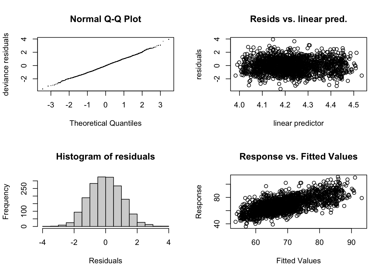
Model Diagnostics
Again, we use gam.check() to evaluate the adequacy of the spline basis dimensions and the overall stability of the fitted GAM. This diagnostic checks whether each smooth term has enough flexibility (via its basis size \(k\)) to capture the underlying pattern in the data, and verifies model convergence, gradient behavior, and Hessian stability.
If a term shows a low k-index (< 1) with a significant p-value, it suggests that the chosen \(k\) is too low and the smooth may be underfitting.
Otherwise, large p-values indicate that the current basis dimension is sufficient for that term.
gam.check(fit)
Method: REML   Optimizer: outer newton
full convergence after 10 iterations.
Gradient range [-0.0002595022,0.0008164376]
(score 1079.705 & scale 1.08843).
Hessian positive definite, eigenvalue range [7.693588e-06,906.0847].
Model rank =  179 / 179

Basis dimension (k) checking results. Low p-value (k-index<1) may
indicate that k is too low, especially if edf is close to k'.

                k'   edf k-index p-value
s(pm25_lag1)  9.00  1.00    1.03    0.93
s(doy)       28.00 13.65    1.02    0.80
s(date2)     99.00 11.11    0.93  <2e-16 ***
s(Temp)       9.00  1.69    1.00    0.51
s(DpTemp)     9.00  1.00    1.00    0.55
s(rmTemp)     9.00  5.42    1.05    0.99
s(rmDpTemp)   9.00  1.00    1.01    0.60
---
Signif. codes:  0 '***' 0.001 '**' 0.01 '*' 0.05 '.' 0.1 ' ' 1
Basis dimension adequacy:
Most smooth terms have high k-index values (~1) and non-significant p-values, indicating that the chosen basis dimensions (\(k\)) were adequate for capturing the data’s complexity.
Potential under-smoothing:
If any term had a lower k-index and significant p-value, suggesting that the basis dimension might be slightly restrictive for long-term trends. Increasing \(k\) could allow more temporal flexibility if needed.
Overall adequacy:
The diagnostic results overall confirm that the spline basis choices and penalization settings are appropriate.
Uncertainty Bands for GAM Smooths
In a GAM, each smooth \(f_j(x)\) is estimated by penalized likelihood. For one smooth with basis vector \(\mathbf{b}(x)\) and coefficients \(\boldsymbol{\beta}_j\), write \[
f_j(x) \;=\; \mathbf{b}(x)^\top \boldsymbol{\beta}_j.
\]
Estimation maximizes a penalized log-likelihood \[
\ell(\boldsymbol{\beta}\,;\,\mathbf{y}) \;-\; \tfrac{1}{2}\sum_j \lambda_j\,\boldsymbol{\beta}_j^\top \mathbf{K}_j \boldsymbol{\beta}_j,
\] where \(\mathbf{K}_j\) encodes curvature of \(f_j\) and \(\lambda_j \ge 0\) controls smoothness.
Near the optimum, a second-order (quadratic) approximation gives an approximately normal sampling distribution for the full coefficient vector \(\boldsymbol{\beta}\): \[
\hat{\boldsymbol{\beta}} \;\approx\; N\!\Big(\boldsymbol{\beta}_{\text{true}},\; \mathbf{V}_{\beta}\Big),
\qquad
\mathbf{V}_{\beta} \;\approx\; \big(\,\hat{\mathbf{I}} \;+\; \sum_j \lambda_j \mathbf{K}_j\,\big)^{-1},
\] where \(\hat{\mathbf{I}}\) is the observed Fisher information from the GLM/GAM fit (for Gaussian models, \(\hat{\mathbf{I}}=\mathbf{X}^\top \mathbf{X}/\hat{\sigma}^2\)).
For the smooth \(f_j\) at a point \(x\), \[
\hat{f}_j(x) \;=\; \mathbf{b}(x)^\top \hat{\boldsymbol{\beta}}_j,
\qquad
\mathrm{SE}\{\hat{f}_j(x)\} \;=\; \sqrt{\,\mathbf{b}(x)^\top \mathbf{V}_{\beta,j}\, \mathbf{b}(x)\,},
\] where \(\mathbf{V}_{\beta,j}\) is the block of \(\mathbf{V}_{\beta}\) for smooth \(j\).
A pointwise 95% interval on the linear predictor scale is therefore \[
\hat{f}_j(x) \;\pm\; 1.96 \times \mathrm{SE}\{\hat{f}_j(x)\}.
\]
If the model uses a link \(g(\mu)=\eta\) (e.g., log for Poisson, logit for binomial), the bands above are for \(\eta\). To present on the response scale, transform:
Poisson/log link: \(\hat{\mu}(x)=\exp\{\hat{\eta}(x)\}\), with delta-method SE if needed.
The penalty adds curvature control and changes the coefficient covariance to \(\big(\hat{\mathbf{I}} + \sum_j \lambda_j \mathbf{K}_j\big)^{-1}\).
Bands on GAM plots come from the approximate normal distribution of \(\hat{f}_j(x)\) via the basis-covariance-basis sandwich \(\mathbf{b}(x)^\top \mathbf{V}_{\beta,j}\mathbf{b}(x)\).
Shaded regions in mgcv plots are pointwise intervals on the linear predictor; they narrow where the data are dense and widen where data are sparse.
Summary
Section
Description
What is the Model?
A Generalized Additive Model (GAM) extends GLMs by allowing each predictor to have its own smooth, potentially nonlinear effect: \(g(\mathbb{E}[Y]) = \beta_0 + \sum_{j=1}^p s_j(X_j)\).
Why Use GAMs?
To capture nonlinear relationships between predictors and outcomes while keeping the model additive and interpretable. Each smooth \(s_j(X_j)\) shows a separate partial effect.
Key Idea
Replace linear terms with penalized splines; the penalty \(\lambda_j \boldsymbol{\beta}_j'\mathbf{K}_j\boldsymbol{\beta}_j\) controls smoothness. Each \(\lambda_j\) is estimated from data (e.g., REML or GCV).
Multiple Smoothers
GAMs combine several smooth functions additively: \(y_i = \beta_0 + g_1(x_i) + g_2(z_i) + \varepsilon_i\), each with its own smoothing parameter.
Uncertainty Bands
Each smooth \(s_j(x)\) is estimated through spline basis coefficients \(\boldsymbol{\beta}_j\), which have a sampling variance–covariance matrix just like regression coefficients. The standard error of the smooth at any \(x\) is obtained by propagating this variance through \(s_j(x) = \mathbf{b}(x)^\top \boldsymbol{\beta}_j\). The plotted shaded regions are pointwise 95% confidence intervals for the smooth function: \(\hat{s}_j(x) \pm 1.96 \times \mathrm{SE}[\hat{s}_j(x)]\), which widen where the curve is less certain and narrow where data are dense.
Model Checking
gam.check() assesses whether basis dimension \(k\) is large enough and whether smooths are over- or under-fitted. A \(k\)-index near 1 indicates adequate flexibility.
Example 1 – Preterm Birth
Logistic GAM with \(s(\text{age})\) reveals a U-shaped age effect on log-odds of preterm birth—highest at youngest and oldest mothers.
Example 2 – Air Pollution
Poisson GAM of daily deaths vs. lagged PM₂.₅ shows nonlinear exposure effects, seasonality, and long-term trend using multiple smooths.
Interpretation
Each smooth \(s_j(X_j)\) displays the partial, nonlinear effect of \(X_j\) on the response scale defined by the link. Shaded bands show uncertainty.
In Summary
GAMs unify splines and GLMs, offering a flexible, interpretable, and data-driven framework for modeling nonlinear effects across multiple predictors.