Gelman & Hill-style regression intuition (figure referenced in class).
Overview & Concepts: In this module you will get a brief review of concepts learned in BIOS 509 including the multiple linear regression (MLR) framework for estimation, interpretation, prediction, and diagnostics. This material will not be included in the labs or quizzes, but is simply a review guide for you to brush up on material needed for Modules 1-3.
Linear regression model in matrix notation
Inference for regression coefficient estimates, expected values, and predictions.
Dummy variables
Effect modification and confounding
Motivation and Examples
Important
Multiple Linear Regression (MLR) is the standard extension of simple linear regression to include two or more predictors.
Goal: quantify how multiple predictors are simultaneously associated with an outcome.
Interpretation: each \(\beta_j\) is the average change in \(y\) for a one-unit change in \(x_{j}\), holding other predictors fixed.
Uses: adjust for confounding, test effect modification (interactions), improve prediction accuracy.
Assumptions: linearity, independence, constant variance (homoscedasticity), and normally distributed errors.
In short: MLR models a continuous outcome as a linear combination of multiple explanatory variables, enabling adjusted and interpretable population-level associations.
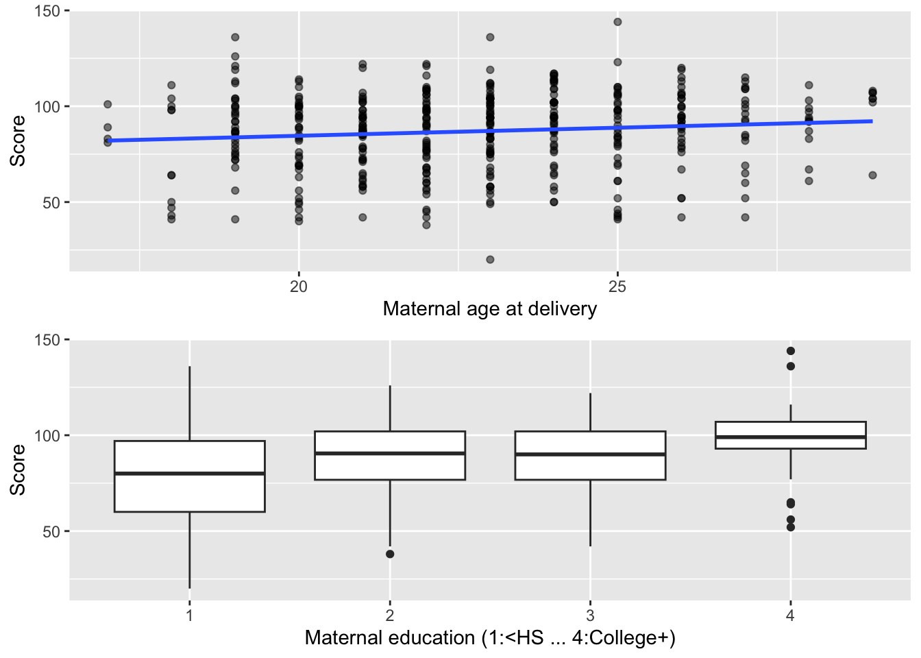
Motivating Example:(NLSY): maternal traits vs. child cognitive score (age 3).
We want to answer the question: What maternal traits are associated with a child’s cognitive score at age 3?
Linear regression is a method that summarizes how the average values of a numerical outcome variable vary over subpopulations (covariate values) defined by linear functions of predictors. Two goals of linear regression:
Prediction of outcome values given fixed predictor values.
Assessment of impact of predictors on the outcome (Estimation).
Let \(y_i\) denote the test score for a given child \(i\). \(age_i\) denotes the corresponding maternal age at delivery for mom \(i\) corresponding to child \(i\), and \(\epsilon_i\) denotes the error term. We will consider the following linear model:
Clearly, we cannot find \(\mathbf{\beta}\) such that this model fits all of our data perfectly.
Model Assumptions:
\(y_i\) is a linear function of \(age_i\), i.e, \(E(\mathbf{Y}) = \mathbf{X\beta} = \mathbf{Age\beta}\) is linear in the \(\beta's\).
\(\beta_0=\) the test score for a child born of a mother at age=0 (not meaningful!)
\(\beta_1=\) average increase in test score associated with one year increase in maternal age.
\(E(\epsilon_i) = 0\) [Expectation of the errors is zero].
Least Squares Solution
Our aim is to find estimates of\(\beta_0\)and\(\beta_1\)that “best” fit the data, but what does “best” mean?
We seek \((\hat{\beta}_0, \hat{\beta}_1)\) that minimizes a loss function.
Our approach is to minimize the sum of squared differences between \(\mathbf{Y}\) and \(\hat{Y} = \mathbf{X\hat{\beta}}\), i.e., this defines the differences between \(\mathbf{Y}\) and the predicted value \(\hat{Y}\) based on a fixed set of \(\beta's\).
Theorem
If \(\mathbf{Y} = \mathbf{X\beta} + \mathbf{\epsilon}\) then the value of \(\hat{\beta}\) that minimizes \((\mathbf{Y - \hat{Y}})^T(\mathbf{Y - \hat{Y}})\) is \(\hat{\beta} = (X'X)^{-1} X'y\).
\(\mathbf{\hat{Y}} = \mathbf{X \hat{\beta}}\) is the fitted (predicted) value.
\(\mathbf{\hat{\epsilon}} = \mathbf{Y} - \mathbf{X\hat{\beta}}\) defines the residual error.
Derivation (matrix calculus)
We estimate \(\hat\beta\) by minimizing the residual sum of squares (RSS):
Differentiate and set to zero (normal equations):\[
\nabla_\beta S(\beta)
= -2\,\mathbf{X}^\top\mathbf{y}
+ 2\,\mathbf{X}^\top\mathbf{X}\,\beta
= \mathbf{0}
\quad\Longrightarrow\quad
\mathbf{X}^\top\mathbf{X}\,\hat\beta
= \mathbf{X}^\top\mathbf{y}.
\]
Solution (full column rank\(\mathbf{X}\): \[
\hat\beta_{OLS}
= (\mathbf{X}^\top\mathbf{X})^{-1}\mathbf{X}^\top\mathbf{y}.
\] For OLS, we have a nice closed-form solution.
Other loss functions or models often require iterative optimization routines.
Orthogonality of residuals: We assume independence between covariate values and residuals.\[
\mathbf{r}=\mathbf{y}-\hat{\mathbf{y}},\qquad
\mathbf{X}^\top\mathbf{r}=\mathbf{0}.
\]
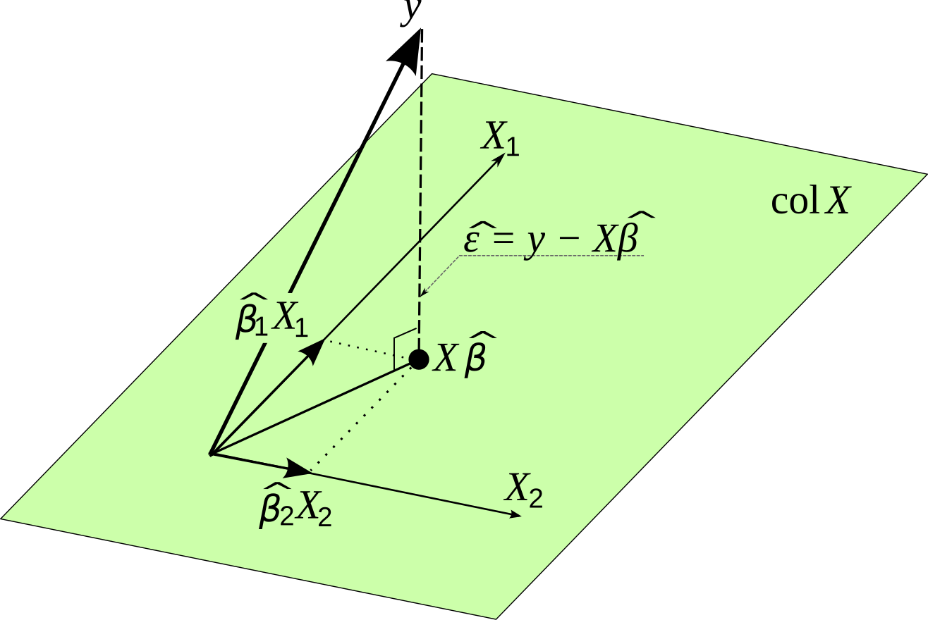
Geometric Interpretation of the OLS estimate
The fitted values \(\hat{y}\) are a linear transformation of \(y\). We see from the figure \(y\) in real space is projected on \(\hat{y}\) in model space.
The HATmatrix is defined as \(\mathbf{H} = \mathbf{X(X^{T} X)^{-1}X^T}\). It is a projection matrix that projects \(y\)\(\rightarrow\)\(\hat{y}\).
\(\hat{\beta}\) is consistent estimation of \(\beta\) under very general assumptions, i.e., \(lim_{n\rightarrow \infty} P(|\hat{\beta} - \beta|>\epsilon) = 0\).
\(\mathbf{\hat{Y}}\) is an unbiased estimator of the mean trend \(\mathbf{X\beta}\).
If \(cov(y) = \sigma^2 I\), the covariance of the estimator \(cov(\mathbf{\hat{\beta}}) = \sigma^2 (X'X)^{-1}\).
Find the\(\operatorname{Cov}(\hat{\beta})\)
We have the linear model \[
\mathbf{y} = \mathbf{X}\beta + \boldsymbol{\epsilon},
\qquad \mathbb{E}[\boldsymbol{\epsilon}] = \mathbf{0},
\qquad \operatorname{Var}(\boldsymbol{\epsilon}) = \sigma^2 \mathbf{I}.
\]
The OLS estimator is \[
\hat{\beta} = (\mathbf{X}^\top \mathbf{X})^{-1}\mathbf{X}^\top \mathbf{y}
= \beta + (\mathbf{X}^\top \mathbf{X})^{-1}\mathbf{X}^\top \boldsymbol{\epsilon}.
\]
The Gauss-Markov Theorem states that, under the classical linear regression assumptions, the OLS estimator is the Best Linear Unbiased Estimator (BLUE) of the coefficients—that is, it has the lowest variance among all linear and unbiased estimators.
\(\mathbf{Y} = \mathbf{X\beta} +\epsilon\)
\(E(\epsilon) = 0\) and \(cov(\epsilon) = \sigma^2 I\)
\(var(\hat{\beta}) = \sigma^2 (X'X)^{-1}\)
\(\hat{\beta}\) is the best (minimum variance) unbiased estimator (BLUE) for \(\mathbf{\beta}\).
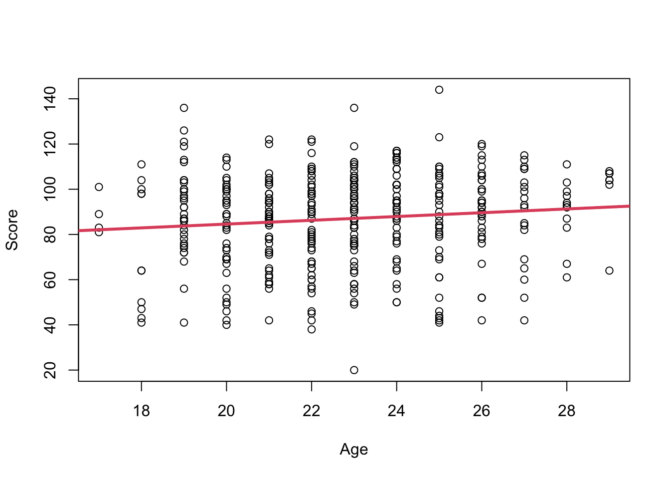
#Visualize the univariate associationplot(score ~ age, data = dat, xlab ="Age", ylab ="Score")abline(beta, lwd =3, col =2)
We see that the regression coefficient estimate for age is \(0.840\). This means that for every 0.840 unit increase in \(age\), there is a 1-unit increase in \(child score\).
Statistical Linear Regression & Inference
The relation between OLS, Normality, and Maximum Likelihood
So far, we have not discussed the distribution of the errors. For OLS we did not need to make any distributional assumption.
\[
\hat{\beta}_{OLS} = (X^TX)^{-1}X^Ty
\]
But for inference (SEs, CIs, p-values), we need to make some distributional assumptions for the errors. Let’s now assume…
\(E(\hat{\sigma}^2_{MLE}) \neq \sigma^2\) so it is NOT unbiased.
An unbiased estimator for \(\sigma^2\) is given by \(s^2 = \frac{1}{n-p} (Y-X\beta)'(Y-X\beta)\).
Summary of OLS vs. MLE approaches
OLS
MLE
Distributional assumption
NONE
Normal \(Y\sim N(X\beta, \sigma^2I)\)
Estimator \(\hat{\beta}\)
\((X'X)^{-1}X'y\)
\((X'X)^{-1}X'y\)
\(cov(\hat{\beta})\)
\(\sigma^2 (X'X)^{-1}\)
\(\sigma^2 (X'X)^{-1}\)
Estimator \(\hat{\sigma}^2\)
Cannot get
\(\frac{1}{n} (Y-X\hat{\beta})'(Y-X\hat{\beta})\) is biased
Estimating the Residual Error
We saw above that the MLE estimator of the residual error: \(\hat{\sigma}^2 = \frac{1} (Y-X\beta)^T(Y-X\beta)\). But this estimator is biased, i.e., \(E(\hat{\sigma}^2) \neq \sigma^2\).
The unbiased estimator of the error variance is the mean squared error (MSE) of the residuals: \(\hat{\sigma}^2 = \frac{1}{n-p} (Y-X\hat{\beta})'(Y-X\hat{\beta})\).
where \(p\) is the number of fitted coefficients (including the intercept). Dividing by \(n-p\) (the residual degrees of freedom) corrects the small-sample bias that would arise if we divided by \(n\).
Its square root, \(\hat\sigma\), is the residual standard error—the typical deviation of observations around the regression line, reported in outcome units.
library(ggplot2)#Here p = 2fit =lm(score ~ age, data = dat)summary(fit)
Call:
lm(formula = score ~ age, data = dat)

Residuals:
    Min      1Q  Median      3Q     Max
-67.109 -11.798   2.971  14.860  55.210

Coefficients:
            Estimate Std. Error t value Pr(>|t|)
(Intercept)  67.7827     8.6880   7.802 5.42e-14 ***
age           0.8403     0.3786   2.219    0.027 *
---
Signif. codes:  0 '***' 0.001 '**' 0.01 '*' 0.05 '.' 0.1 ' ' 1

Residual standard error: 20.34 on 398 degrees of freedom
Multiple R-squared:  0.01223,   Adjusted R-squared:  0.009743
F-statistic: 4.926 on 1 and 398 DF,  p-value: 0.02702
#Can we confirm this manuallyyhat = fit$fitted.values #Predicted Valuesy = dat$score #Observed ValuesN =length(y)P=2#number columns in design matrixsq_error = (y-yhat)^2#Squared errorssigma_squared_est <-sum(sq_error)/(N-P) #Unbiased est of the variancesigma_est =sqrt(sigma_squared_est) #Unbiased est of the std. errorsigma_est
[1] 20.34027
Indeed we see that the estimated residual standard error is \(20.3\). But what does this really mean?
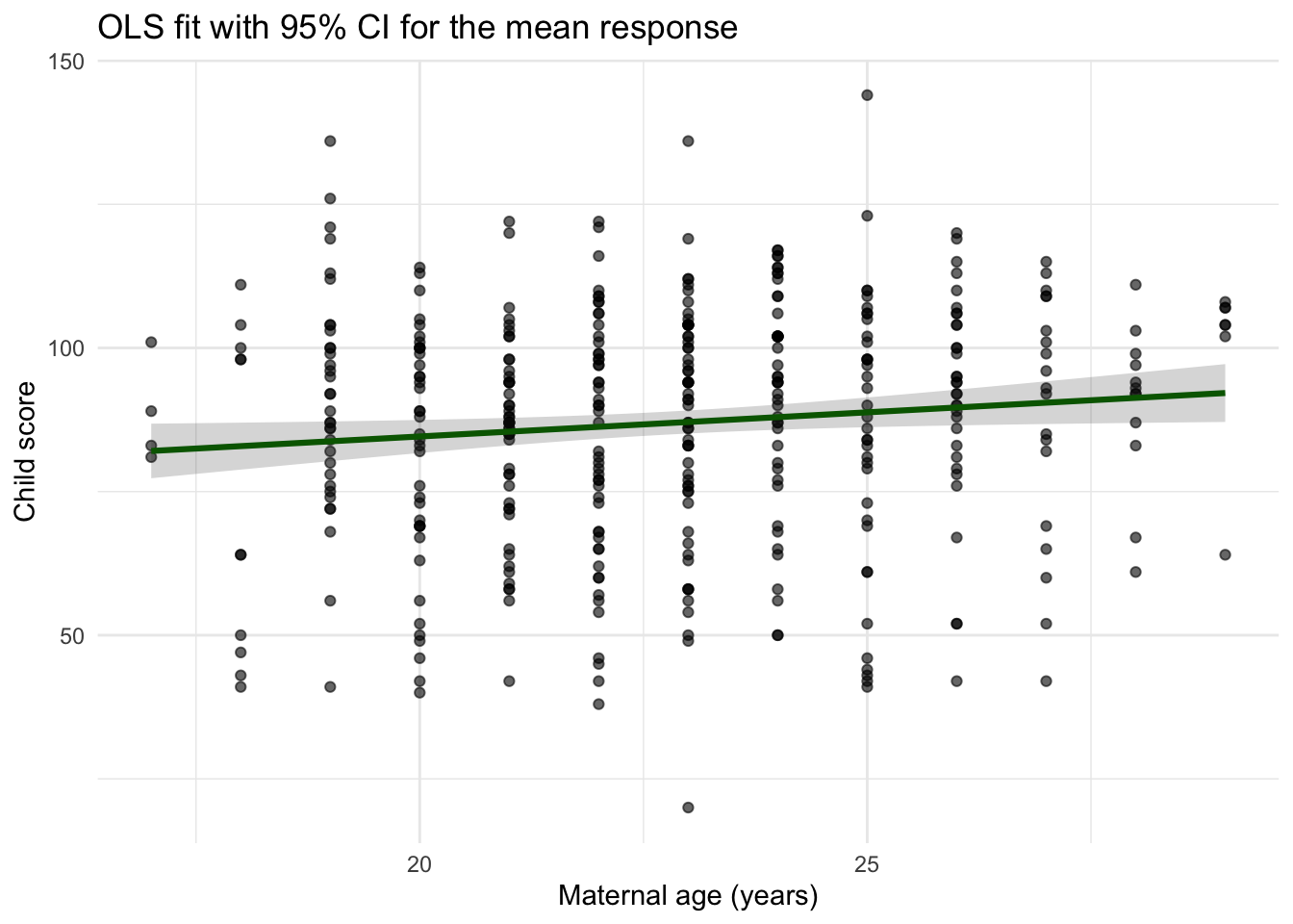
We can visualize uncertainty in the regression line (mean). The pointwise 95% confidence band for the mean at covariate value \(x\) is:
#Include 95% confidence intervals in your summarynd <-data.frame(age =seq(min(dat$age), max(dat$age), length.out =200))ci <-as.data.frame(predict(fit, newdata = nd, interval ="confidence", level =0.95))plt <-cbind(nd, ci)ggplot() +geom_point(data = dat, aes(age, score), alpha =0.6) +geom_ribbon(data = plt, aes(x = age, ymin = lwr, ymax = upr), alpha =0.2) +geom_line(data = plt, aes(x = age, y = fit), linewidth =1.1, color ="darkgreen") +labs(x ="Maternal age (years)", y ="Child score",title ="OLS fit with 95% CI for the mean response") +theme_minimal()
Model Interpretation: A one year increase in mother’s age at delivery was associated with a 0.84 (p-value= 0.027) increase in the child’s average test score, where test score was measured at age 3. The association was statistically significant at a type I error rate of 0.05.
There was considerable heterogeneity in test scores \((\hat{\sigma} = 20.34)\). Therefore, the regression model does not predict individual test scores well \((R^2 = 0.012)\). 1.2% of variances is explained by mother’s age.
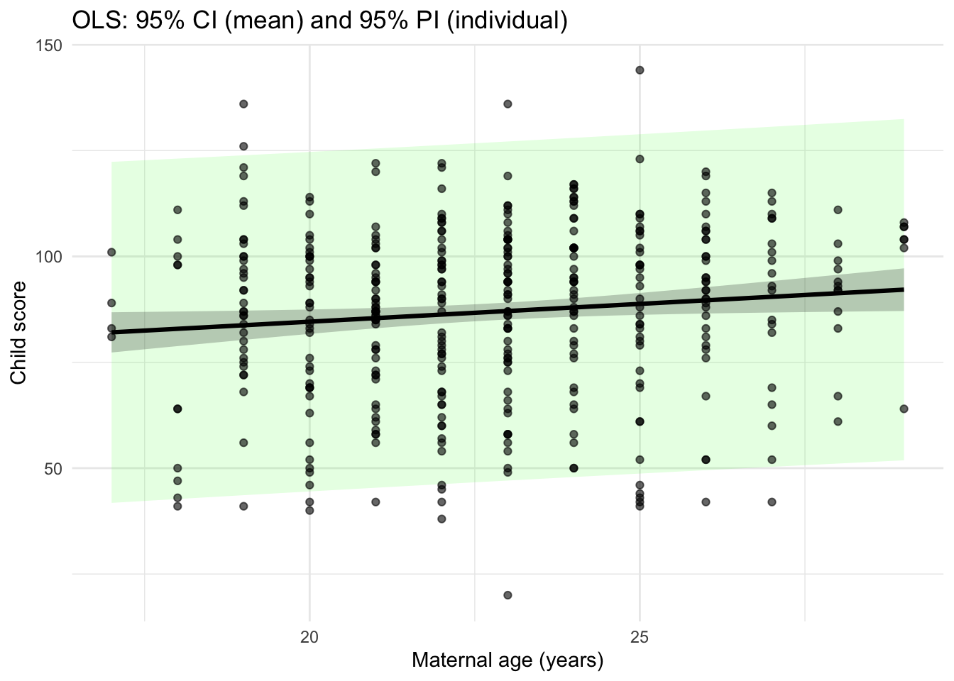
Prediction Interval for a New Observation
Let \(\tilde{y}_i\) be a new observation with covariate value \(age_i\). How can you obtain its predictive uncertainty? We want to capture the uncertainty in our predicted estimate of the expected value \(\hat{y}_i = X\hat{\beta}\) PLUS the uncertainty due to measurement error \(\epsilon_i\).
From this derivation we can see that \(\tilde{\sigma}^2 \geq \hat{\sigma}^2\). So the 95% prediction interval is going to be wider than the 95% confidence interval.
The approximate 95% prediction interval is given by \(\tilde{y}_i \pm 1.96 \tilde{\sigma}\).
fit <-lm(score ~ age, data = dat)# 2) Make a smooth grid over agend <-data.frame(age =seq(min(dat$age), max(dat$age), length.out =200))# 3) Get intervalsci <-as.data.frame(predict(fit, newdata = nd, interval ="confidence", level =0.95))pi <-as.data.frame(predict(fit, newdata = nd, interval ="prediction", level =0.95))plot_df <-cbind(nd,fit = ci$fit,lwr_ci = ci$lwr, upr_ci = ci$upr,lwr_pi = pi$lwr, upr_pi = pi$upr)# 4) Plot: points, prediction band (wider), mean CI band (narrower), fitted lineggplot() +# prediction band (wider)geom_ribbon(data = plot_df,aes(x = age, ymin = lwr_pi, ymax =upr_pi), alpha =0.12, fill ="green") +# mean CI band (narrower)geom_ribbon(data = plot_df,aes(x = age, ymin = lwr_ci, ymax =upr_ci),alpha =0.25) +# fitted linegeom_line(data = plot_df,aes(x = age, y = fit),linewidth =1.1) +# points last so they sit on topgeom_point(data = dat,aes(x = age, y = score),alpha =0.6) +labs(x ="Maternal age (years)", y ="Child score",title ="OLS: 95% CI (mean) and 95% PI (individual)") +theme_minimal()
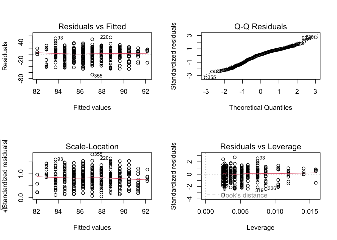
Model Diagnostics
Residual vs. Fitted
\(\hat{\epsilon}_i\) should be independent of \(\hat{y}_i\), i.e., no patterns.
Linearity: Red line should be flat, ie banded around 0.
Constant variance (homoscedasticity).
Normal Q-Q Plot
Standardized residual \(\hat{\epsilon}_i/ (\hat{ \sigma} \sqrt{1-h_{ii}})\) should be a standard normal.
We expect the points to follow a straight line, Check non-normality, particularly skewed tails.
Scale-Location
Similar to residual vs fitted, but use standardized residual. Diagnose heteroscedasticity (eg red line increasing).
Residual vs Leverage
Leverage \(h_{ii}\) is how far away \(x_i\) is from other \(x_j\) where \(h_{ii} = \frac{\partial \hat{y}_i}{\partial y_i}\).
Cook’s Distance: measures how much model changes when remove \(ith\) point; >1 is problematic.
par(mfrow=c(2,2))plot(fit)
Hypothesis Testing
With the linear regression model established, we now turn to hypothesis testing to determine whether the relationships observed between the independent and dependent variables are statistically significant.
(Intercept): \(H_0 : \beta_0 = 0\) when \(age =0\). In other words test scores are equal to zero for a mother at \(age=0\) versus \(H_a: \beta_0 \neq 0\).
Age: \(H_0: \beta_1=0\) In words, the slope of age is equal to zero or there is no linear effect. \(H_a: \beta_1 \neq 0\) if there is a significant linear effect.
For a given covariate \(\beta_j\), we make the following assumption:
The test statistic follows a \(t\)-distribution under the null hypothesis:
\[
t = \frac{\hat{\beta}_j}{\mathrm{SE}(\hat{\beta}_j)} \sim t_{n - p}
\]
We compare this statistic to critical values of the \(t\)-distribution or use its corresponding p-value to decide whether to reject \(H_0\).
summary(fit)
Call:
lm(formula = score ~ age, data = dat)

Residuals:
    Min      1Q  Median      3Q     Max
-67.109 -11.798   2.971  14.860  55.210

Coefficients:
            Estimate Std. Error t value Pr(>|t|)
(Intercept)  67.7827     8.6880   7.802 5.42e-14 ***
age           0.8403     0.3786   2.219    0.027 *
---
Signif. codes:  0 '***' 0.001 '**' 0.01 '*' 0.05 '.' 0.1 ' ' 1

Residual standard error: 20.34 on 398 degrees of freedom
Multiple R-squared:  0.01223,   Adjusted R-squared:  0.009743
F-statistic: 4.926 on 1 and 398 DF,  p-value: 0.02702
TEST YOUR KNOWLEDGE
Let \(H=X(X'X)^{-1}X'\) and let \(\hat{Y} = HY\). Then \(H\hat{Y} = ?\)
Show the derivation for \(cov(\hat{\beta})\).
What is the unbiased estimator of \(\sigma^2\)?
The unbiased estimator for \(\sigma^2\) contains a parameter \(p\). What does \(p\) represent?
Below code is given to simulate data from a “true” model. Run the code to get simulated quantities of covariates \(X\) and outcomes \(Y\).
What is the “true” intercept in the below simulation?
What is the “true” covariate coefficient value in the below simulation?
Fit the linear model. Find the estimates of the \(\beta’s\) and global variance \(\sigma^2\).
Interpret the findings of the model in terms of null versus alternative hypotheses.
Create diagnostic plots and determine if model assumptions have been met.
#Set seed for reproducibilityset.seed(1232)#Set the "true" values of the betas.beta0 =0.1beta1 =0.5beta2 =-0.2#Simulated data from two normalsx1 <-rnorm(n=100, 0, 2)x2 <-rnorm(n=100, 5, 5)error <-rnorm(n=100, 0, 1)#Generate the simulated y valuesX =cbind(1, x1, x2)Beta =c(beta0, beta1, beta2)Y = X %*% Beta + error###Finish this code to run the proposed model and diagnostics.
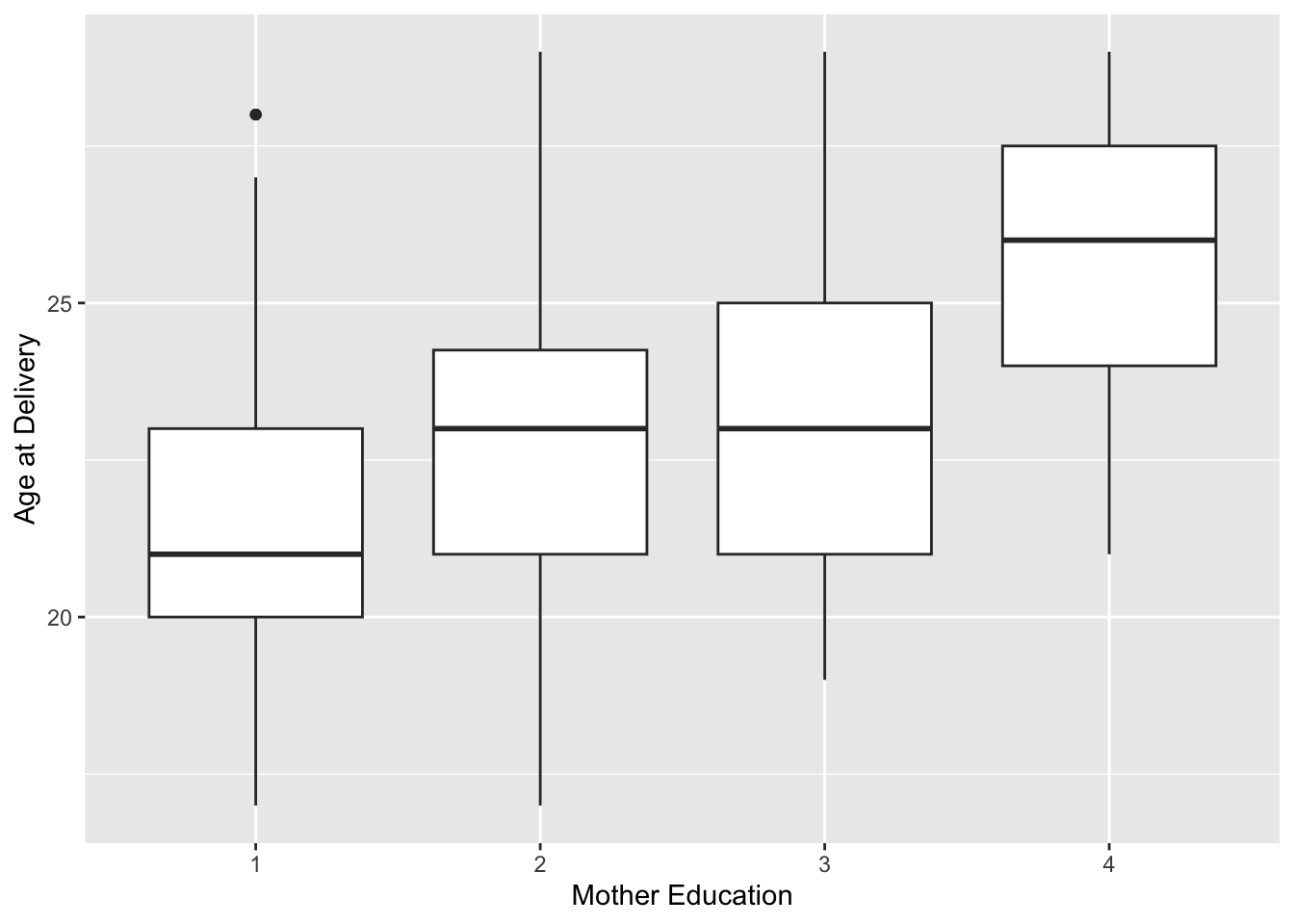
Confounding
We found that older mothers had children on average with higher test scores. However, higher maternal education was associated with higher age as shown below.
How do we estimate the age association with outcome accounting for the effect (confounding) of education?
ggplot(dat) +geom_boxplot(aes(as.factor(edu),age)) +labs(x ="Mother Education", y="Age at Delivery")
Confounding
Causes spurious correlation.
Referred to as “omitted variable bias”
We want to control/account for confounding associations!
How do we account for confounding?
Include confounders in the regression equation\(\rightarrow\) MULTIPLE LINEAR REGRESSION: \(y \sim x+z\)
Assumptions of linear regression plus omitted variable assumption:
Residuals are independent AND normal.
Global variance (homoscedasticity).
Linearity of all included covariates.
All variables that are not included in the model have coefficient equal to zero (omitted variable bias = 0).
fit =lm(dat$score ~ E1 + E2 + E3 + E4 -1) #use -1 to remove the interceptsummary(fit)
Call:
lm(formula = dat$score ~ E1 + E2 + E3 + E4 - 1)

Residuals:
   Min     1Q Median     3Q    Max
-58.45 -12.70   1.61  15.23  57.55

Coefficients:
   Estimate Std. Error t value Pr(>|t|)
E1   78.447      2.159   36.33   <2e-16 ***
E2   88.703      1.367   64.88   <2e-16 ***
E3   87.789      2.284   38.44   <2e-16 ***
E4   97.333      3.831   25.41   <2e-16 ***
---
Signif. codes:  0 '***' 0.001 '**' 0.01 '*' 0.05 '.' 0.1 ' ' 1

Residual standard error: 19.91 on 396 degrees of freedom
Multiple R-squared:  0.9508,    Adjusted R-squared:  0.9503
F-statistic:  1913 on 4 and 396 DF,  p-value: < 2.2e-16
What does each element of \(\beta\) vector mean?
\(\hat{\beta}_1\) is equivalent to taking the average of scores for kids with mother’s \(edu=1\). So each \(\hat{\beta}\) is equivalent to calculating the mean IQ for each education group.
Approach 2: Intercept plus three indicators for groups 2,3, and 4.
Call:
lm(formula = dat$score ~ factor(dat$edu))

Residuals:
   Min     1Q Median     3Q    Max
-58.45 -12.70   1.61  15.23  57.55

Coefficients:
                 Estimate Std. Error t value Pr(>|t|)
(Intercept)        78.447      2.159  36.330  < 2e-16 ***
factor(dat$edu)2   10.256      2.556   4.013 7.18e-05 ***
factor(dat$edu)3    9.342      3.143   2.973  0.00313 **
factor(dat$edu)4   18.886      4.398   4.294 2.21e-05 ***
---
Signif. codes:  0 '***' 0.001 '**' 0.01 '*' 0.05 '.' 0.1 ' ' 1

Residual standard error: 19.91 on 396 degrees of freedom
Multiple R-squared:  0.05856,   Adjusted R-squared:  0.05142
F-statistic:  8.21 on 3 and 396 DF,  p-value: 2.59e-05
\(\hat{\beta}\) represents the difference in average score with respect to the \(edu=1\) group., i.e., 10.256 is the average difference between no high school group and high school group.
Variance Inflation Factors
One must always be on the lookout for issues with multicollinearity!
The general issues is that when two variables are highly correlated, it is hard to disentangle their effects.
Mathematically, the standard errors are inflated. Suppose we have a design matrix \(\mathbf{X} = [x_1, ..., x_p]\) and we want to calculate the variance inflation factor (VIF). We regress \(x_1\) against \(x_2, ..., x_p\).
Let \(R_1^2\) be the associated R-squared for \(x_1\). Then \(VIF_1 = \frac{1}{1-R_1^2}\).
It can be shown that \(Var(\hat{\beta}_j) = VIF_j \cdot \frac{\sigma^2}{(n-1)s_{x_j}^2}\).
Different rules of thumb \(VIFs>5\) are cause for concern.
library(car)
Loading required package: carData
Attaching package: 'car'
The following object is masked from 'package:dplyr':

    recode
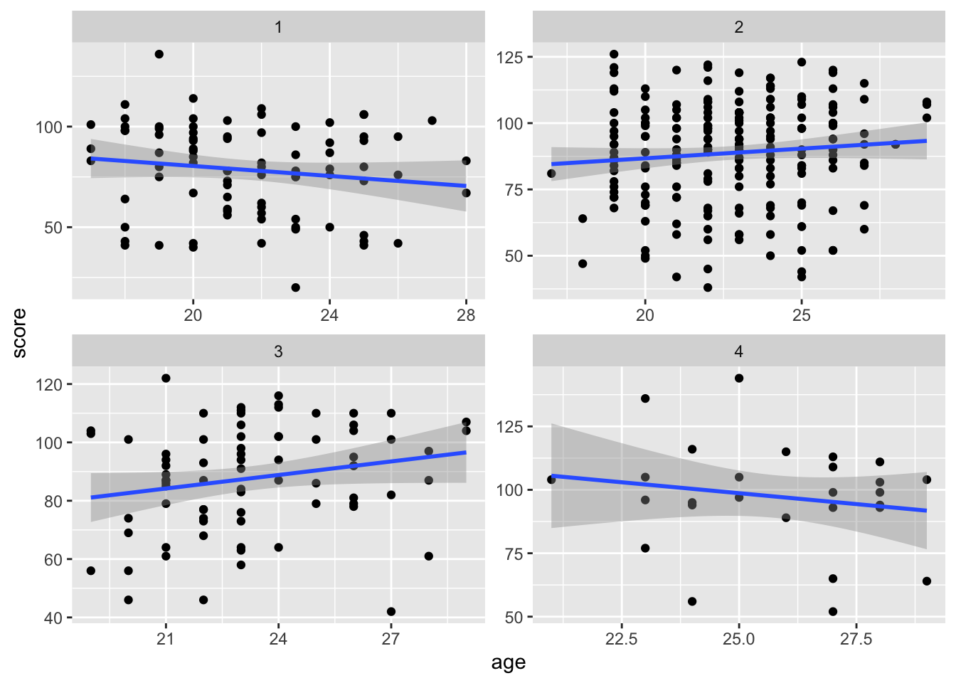
To test whether the interaction was significant, look at whether the inclusion of the interaction significantly “improved” model fit.
\(H_0\): The interaction between education and age does not improve model fit.
\(H_A\): The interaction improves model fit.
Suppose we want to choose between these two models, i.e., Full model vs. Reduced model. We use the F-statistic:
F-statistic to perform model comparison
The F statistic is a ratio of two chi-square distributions to test whether the full model gives additional information, e.g., does \(\beta_5 = \beta_6 = \beta_7 =0\)?
\[
F = \frac{ \text{RSS}_{\text{reduced}} - \text{RSS}_{\text{full}} }{ p_{\text{full}} - p_{\text{reduced}} } \Bigg/ \frac{ \text{RSS}_{\text{full}} }{ n - p_{\text{full}} },.
\] Another parametrization for the F-test is given by:
fit_inter =lm(score ~factor(edu) * age, data = dat) #Full Modelfit_nointer =lm(score~factor(edu) + age, data = dat) #Reduced Modelanova(fit_nointer, fit_inter)
Analysis of Variance Table

Model 1: score ~ factor(edu) + age
Model 2: score ~ factor(edu) * age
  Res.Df    RSS Df Sum of Sq      F  Pr(>F)
1    395 156733
2    392 153857  3    2876.5 2.4429 0.06376 .
---
Signif. codes:  0 '***' 0.001 '**' 0.01 '*' 0.05 '.' 0.1 ' ' 1
Overall, there is only limited statistical evidence of an interaction!
Summary
Section
Description
Model (MLR)
\(\mathbf y=\mathbf X\beta+\boldsymbol\epsilon\), with \(E[\boldsymbol\epsilon]=\mathbf 0\), \(\operatorname{Var}(\boldsymbol\epsilon)=\sigma^2\mathbf I\). Each \(\beta_j\) is an adjusted effect.
\(E[\hat\beta]=\beta\); \(\operatorname{Cov}(\hat\beta)=\sigma^2(\mathbf X^\top\mathbf X)^{-1}\); residuals are orthogonal to columns of \(\mathbf X\).
Normality for inference
For SEs/CIs/p-values assume \(\boldsymbol\epsilon\sim\mathcal N(\mathbf 0,\sigma^2\mathbf I)\). Point estimates don’t require normality.
Residual variance
\(\hat\sigma^2=\mathrm{SSE}/(n-p)\) with \(\mathrm{SSE}=\sum (y_i-\hat y_i)^2\), \(p\) includes the intercept. \(\hat\sigma\) = residual standard error.
Mean CI & Prediction PI
95% CI bands quantify uncertainty in the mean\(\hat y(x)\); 95% PI adds error variance and is wider (for new observations).
Diagnostics
Residuals vs fitted (linearity/variance), Normal Q–Q (normality), Scale–Location (homoscedasticity), Residuals vs leverage/Cook’s \(D\) (influence).
Hypothesis tests
\(t\)-tests for individual coefficients (e.g., slope of age). Partial \(F\)-tests for blocks of terms (e.g., interactions).
Confounding
Adjust by including confounders in \(\mathbf X\) to obtain population-level, adjusted associations.
Categorical predictors
Use \(k-1\) indicators with an intercept (reference coding) for group mean differences.
Multicollinearity (VIF)
\(\text{VIF}_j = 1/(1-R_j^2)\); values \(\gtrsim 5\) are a concern (rule of thumb in these notes).
Interactions
Add terms like \(x:\text{group}\) for group-specific slopes; without interactions slopes are common across groups.
F-test of interaction
Compare full vs reduced models to test whether interaction terms improve fit.