In Module 4B, we learned about parametric splines, where we fit piecewise polynomial segments joined at knots. These splines required us to choose both the number and location of the knots.
If we choose too few knots, the fit is too rigid and misses local patterns (high bias). If we choose too many knots, the spline can overfit and capture random noise (high variance).
Question: Is there a way to include many knots for flexibility but automatically control how wiggly the curve becomes?
Answer: Yes — by adding a penalty for roughness. This leads to penalized splines and smoothing splines.
Penalized Regression Framework: The Idea Behind Penalized Splines
and approximate the unknown function \(g(x)\) using a flexible basis representation with large fixed \(K\) is unknown.
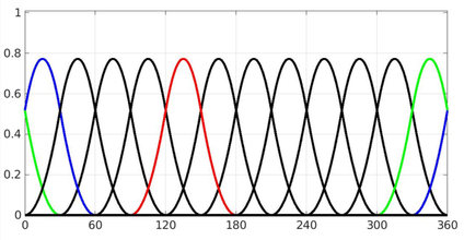
Instead of forcing \(g(x)\) to have a specific parametric form, we approximate it using many basis functions:
\[
g(x) = \sum_{k=1}^K \beta_k b_k(x)
\] In Module 4B, we chose \(K\) by deciding where to put knots. Here we take a different approach.
The main idea is we start with a lot of knots. This ensures we will not miss important fine-scale behavior. Next, we assume most of the knots are not useful and shrink their coefficients towards zero. We determine the amount of shrinkage based on some criteria (.e.g, CV, GCV, AIC). Benefits of this approach:
Knot placement is not important if the number if dense enough, but be cautious for overfitting.
Shrinking most coefficients to zero will stabilize model estimation similar to performing variable selection.
Data decide how much flexibility is needed.
Penalized Least Squares (PLS)
Intuition: Ordinary least squares minimizes the sum of squared residuals. Penalized least squares adds a second term that discourages unnecessary complexity in the fitted function.
To estimate \(g(x)\) we minimize a penalized residual sum of squares:
The second term \(J(g)\) measures the roughness of the function.
\(\lambda\) controls the tradeoff between fit and smoothness.
Note
Interpretation of \(\lambda\):
Small \(\lambda\) → minimal penalty → curve follows data closely (wiggly fit).
Large \(\lambda\) → heavy penalty → smoother curve (may miss fine details).
Constrained vs. Penalized Form
There are two equivalent ways to control how smooth the estimated function is: we can either place a hard limit on its wiggliness (constrained form) or penalize wiggliness directly in the objective function (penalty form).
Here we allow the curve to fit the data but restrict its total roughness, i.e., fit the data well, but don’t let the function be too rough. The constant \(c\) sets an upperbound on how wiggly \(g(x)\) can be. This is computationally inconvenient.
Here, we trade off between fit and smoothness. The constant \(\lambda\) acts as a Lagrange multiplier linked to constraint \(c\), i.e., fit the data and smoothness simultaneously-balancing them through \(\lambda\).
Examples of PLS Using Different Penalties
Penalized Least Squares (PLS) can take different forms depending on what we choose to penalize
Ridge regression- \(J(g)\) penalizes the size of the coefficients.
\[
J(g) = \sum_{m=1}^M \beta_m^2 = ||\beta||_2^2 \leq C
\]
where \(||\beta||_2\) is the L2-Norm and \(C\) is a positive constant. Ridge regression using the \(L2-\) penalty which does not induce sparsity because is does not set \(\beta's\) exactly to 0.
L2 Definition
The L2 norm, also called the Euclidean norm, is a measure of the magnitude (or length) of a vector in Euclidean space. It is defined as:
Geometric Interpretation: The L2 norm corresponds to the Euclidean distance from the origin to the point \(\mathbf{v}\) in \(n\)-dimensional space. For a 2D vector \(\mathbf{v} = [x, y]\), the L2 norm is:
\[
\|\mathbf{v}\|_2 = \sqrt{x^2 + y^2}
\]
This is the standard distance formula in 2D geometry.
Lasso- \(J(g)\) penalizes the size of the coefficients using the \(L_1\) norm.
\[
J(g) = \|\beta\|_1 \leq C,
\]
where \(\|\beta\|_1\) is the L1-Norm and \(C\) is a positive constant.
LASSO applies an \(L1\) penalty, which encourages sparsity in the coefficients.
Unlike Ridge regression, Lasso can set some \(\beta\)’s exactly to 0, effectively performing variable selection while also regularizing the model.
Scalability: For a scalar \(c\): \[
\|c\mathbf{v}\|_1 = |c| \cdot \|\mathbf{v}\|_1
\]
Triangle Inequality: For any vectors \(\mathbf{u}\) and \(\mathbf{v}\): \[
\|\mathbf{u} + \mathbf{v}\|_1 \leq \|\mathbf{u}\|_1 + \|\mathbf{v}\|_1
\]
Geometric Interpretation:
The L1 norm corresponds to the sum of absolute distances along each axis from the origin to the point \(\mathbf{v}\).
In 2D, this is the total “city-block distance” you’d travel along grid lines: \[
\|\mathbf{v}\|_1 = |x| + |y|
\]
The L1 constraint region forms a diamond shape in 2D, which causes some coefficients to hit exactly zero—unlike the circular constraint region in Ridge regression.
Connection to Penalized Splines: Ridge and Lasso are both examples of the penalized least squares framework:
\[
\sum_i (y_i - g(x_i))^2 + \lambda J(g)
\] In these cases, \(J(g)\) penalizes the size of the coefficients.
PLS: Moving from Constraints to Penalties
For Penalized Spline, the same principle is used — but \(J(g)\) penalizes the roughness of the function, rather than the size of the coefficients. In other words, the penalty smooths the entire fitted curve, not just the individual coefficients.
Mathematically, this is achieved y penalizing the integrated squared second derivative: \[
J(g) = \int [g''(x)]^2 dx
\]
This quantity measures how rapidly the function \(g(x)\) bends or changes curvature (wiggliness). Large values of \(J(g)\) indicate a very wiggly function, while smaller values correspond to smoother curves.
By adding \(\lambda J(g)\) to our objective function, we control the trade-off between smoothness and fit.
Deriving the Penalized Spline Solution
We now express the penalized spline problem in matrix form. This will show that the solution has the same algebraic form as ridge regression, even though the penalty targets curvature rather than coefficient size.
Let \(\mathbf{B}\) be the basis matrix (each column a basis function evaluated at all \(x_i\)), and let \(\boldsymbol{\beta}\) be the corresponding coefficient vector. Then the PLS criterion can be written as
where \(\mathbf{K}\) is a known penalty matrix that encodes curvature or “wiggliness” of the fitted function.Typically, \(\mathbf{K}\) is derived from \(\int b_k''(x)b_l''(x)dx\), so that large curvature is penalized.
Derivation of the Closed-Form Solution
Optimization Problem
We seek to minimize the penalized least squares criterion:
\(\lambda = 0\):
The penalty disappears and \(\hat{\boldsymbol{\beta}}\) reduces to the ordinary least squares (OLS) estimate.
\(\lambda \to \infty\):
The penalty dominates; higher-order coefficients shrink toward zero, producing a smoother (even linear) function.
Intercept and linear terms (\(\beta_0\), \(\beta_1\)) are usually not penalized, allowing the fitted spline to capture the overall level and trend freely. |
Fitting Penalized Splines in R
Let’s revisit our NYC daily mortality data. We can use a penalized spline on date_num:
library(splines)library(MASS)library(mgcv)# Load dataload(file.path(getwd(), "data", "NYC.RData")) # expects object `health`# Ensure date is numeric for bs(); keep original for labelinghealth$date_num <-as.numeric(health$date)# --- 1. Unpenalized spline (ordinary regression spline) ---fit_unpen <-lm(alldeaths ~bs(date_num, df =40), data = health)# --- 2. Penalized spline (penalized B-spline, ps basis) ---fit_pen <-gam(alldeaths ~s(date_num, k =40, #k=40 is defaultybs ="ps"),data = health, method ="GCV.Cp")# --- Plot comparison ---plot(health$date_num, health$alldeaths, pch =16, cex =0.6,col ="gray50", main ="Penalized vs Unpenalized Splines",xlab ="Date (numeric)", ylab ="All Deaths")# Add unpenalized spline fit (red, more wiggly)lines(health$date_num, fitted(fit_unpen), col ="red", lwd =2)# Add penalized spline fit (blue, smoother)lines(health$date_num, fitted(fit_pen), col ="blue", lwd =2)legend("topright", legend =c("Unpenalized (OLS spline, λ = 0)","Penalized (GCV-selected λ)"),col =c("red", "blue"), lwd =c(1.5, 3), lty =c(2, 1), bty ="n")
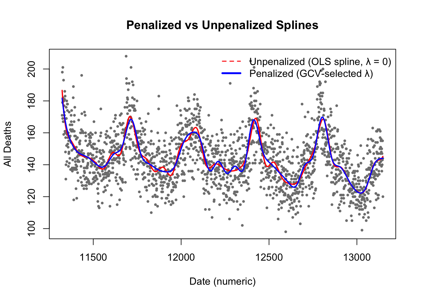
The gray points show daily (or observed) values of all deaths in NYC.
The red curve represents the unpenalized spline fit.
It follows the data very closely, producing a wiggly fit.
This corresponds to λ = 0, i.e., no smoothness penalty.
High flexibility → low bias, high variance.
The blue curve represents the penalized spline fit.
The penalty term discourages excessive curvature, yielding a smoother trend.
The model automatically chooses the optimal λ by REML (or GCV).
The comparison shows that penalization reduces random wiggles while retaining major seasonal patterns. Conceptually, the penalty shrinks the coefficients associated with high-order basis functions toward zero— just as predicted by the ridge-type matrix solution\(\hat{\boldsymbol{\beta}} = (\mathbf{B}'\mathbf{B} + \lambda\mathbf{K})^{-1}\mathbf{B}'\mathbf{y}\).
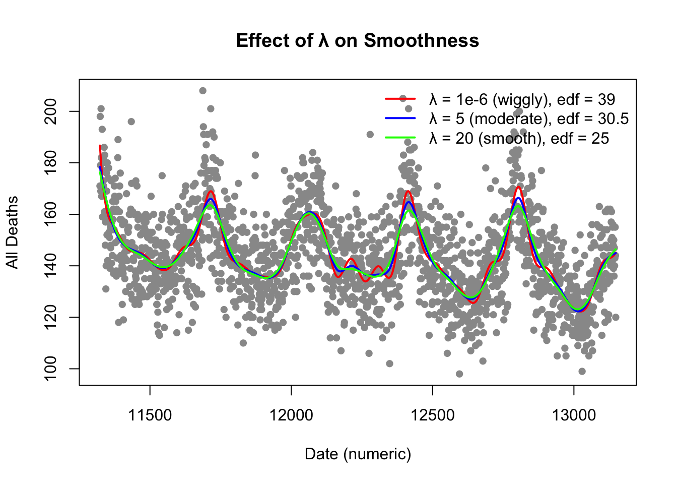
So far, we’ve seen that \(\lambda\) controls the trade-off between fit and smoothness: Small \(\lambda\) → minimal penalty → very flexible (wiggly) curve. Large \(\lambda\) → heavy penalty → smoother curve (possibly underfit). But how do we choose the “right” amount of smoothing? We need a method to balance goodness of fit and model complexity.
The smoothing parameter\(\lambda\) controls the trade-off between fit and smoothness (i.e., the bias–variance tradeoff). Choosing \(\lambda\) too small leads to an overfitted, wiggly curve; choosing it too large leads to an oversmoothed, biased curve.
You can think of it like the story of “Goldie-Locks and the three Bears”:
Too little smoothing (small \(\lambda\)) → the fit is too rough (high variance).
Too much smoothing (large \(\lambda\)) → the fit is too flat (high bias).
The “just right”\(\lambda\) finds the balance between flexibility and stability.
To select \(\lambda\), we can minimize the Generalized Cross-Validation GCV criterion, a computational shortcut to LOO validation:
Small \(\lambda\) → edf ≈ number of parameters (flexible fit).
Large \(\lambda\) → edf ≈ 2 (approaches a line).
edf quantifies the model’s effective flexibility—how many ‘free bends’ the spline is allowed to have.
The numerator is the mean squared error (avg lack of fit).
The denominator corrects for model complexity (effective degrees of freedom).
\(\lambda\) that minimizes the GCV achieves the “just right” fit.
GCV provides an automatic, data-driven way to select the smoothness level.
Coming Back to Our Model Findings
Now that we understand how GCV selects the smoothing parameter and how the effective degrees of freedom (edf) quantify smoothness, we can interpret our fitted penalized spline model:
The model was fit using (GCV) to choose the optimal smoothing parameter \(\lambda\).
GCV automatically balances model fit and smoothness.The GCV score = 175.5 and estimated scale = 171.9 quantify residual variability and model adequacy.
The estimated smooth term s(date_num) has effective degrees of freedom (edf) = 36.48 (out of 40 possible), meaning the fitted curve is fairly flexible but still penalized to avoid overfitting.
The smooth term is highly significant (F = 36.83, p < 2 × 10⁻¹⁶), indicating a strong nonlinear temporal pattern in daily deaths.
The intercept = 143.9 represents the estimated average number of deaths (baseline level) after centering effects.
The model explains about 44 % of the total variability in the outcome
(Deviance explained = 44 %, R²₍adj₎ = 0.43), which is typical for real-world time-series mortality data.
A smoothing spline is a special case of the penalized spline where we place a knot at every unique \(x_i\) but penalize curvature to prevent overfitting. The estimation problem becomes:
where \(\lambda\) controls the trade-off between fidelity to the data and smoothness of the curve.
Small \(\lambda\) → the curve follows the data closely (wiggly).
Large \(\lambda\) → the curve becomes smoother, approaching a straight line.
The solution \(g(x)\) can be shown (via calculus of variations) to be a natural cubic spline with knots at all unique \(x_i\).
In practice, smoothing splines are conceptually elegant but computationally intensive for large \(n\), so penalized B-splines (P-splines) are preferred in most applications.
Smoothing splines illustrate the extreme limit of penalized splines—maximal flexibility regulated entirely by λ.
Summary
Section
Description
Penalized Regression Framework
Estimates \(g(x)\) by minimizing the penalized least squares criterion: \[\text{PLS}(\lambda) = \sum_{i=1}^{n}(y_i - g(x_i))^2 + \lambda J(g).\] The first term measures goodness of fit; the second penalizes roughness.
Matrix Formulation
In matrix form, the ridge-type estimator is \[\hat{\boldsymbol{\beta}} = (\mathbf{B}'\mathbf{B} + \lambda \mathbf{K})^{-1}\mathbf{B}'\mathbf{y}.\] Penalization shrinks coefficients associated with high curvature toward zero.
Penalty Matrix\(\mathbf{K}\)
Encodes curvature or “wiggliness” through \[K_{kl} = \int b_k''(x)b_l''(x)\,dx.\] Large curvature implies larger penalty and smoother estimated functions.
Smoothing Parameter\(\lambda\)
Controls the bias–variance tradeoff: Small \(\lambda\) → wiggly, flexible fit (low bias, high variance). Large \(\lambda\) → smooth, stable fit (high bias, low variance).
Smoother Matrix\(\mathbf{S}_\lambda\)
Maps observed values to fitted values: \[\hat{\mathbf{y}} = \mathbf{S}_\lambda \mathbf{y}, \quad \mathbf{S}_\lambda = \mathbf{B}(\mathbf{B}'\mathbf{B} + \lambda\mathbf{K})^{-1}\mathbf{B}'.\] Captures how each observation influences its own fitted value.
Effective Degrees of Freedom (edf)
Measures model flexibility: \[\text{edf} = \text{trace}(\mathbf{S}_\lambda).\] Small \(\lambda\) → large edf (many bends); large \(\lambda\) → small edf (smoother curve).
Choosing\(\lambda\): GCV Criterion
The optimal \(\lambda\) is chosen by minimizing the Generalized Cross-Validation (GCV) statistic: \[\text{GCV}(\lambda) = \frac{\frac{1}{n}\sum_i (y_i - \hat{y}_i)^2}{\left[1 - \frac{\text{trace}(\mathbf{S}_\lambda)}{n}\right]^2}.\] Provides a data-driven balance between fit and smoothness.
Smoothing Spline (Limit Case)
When knots are placed at every unique \(x_i\), the penalized spline becomes a smoothing spline: \[\min_g \sum_i (y_i - g(x_i))^2 + \lambda \int [g''(x)]^2 dx.\] Produces a globally smooth curve that still adapts to local structure.
Interpretation
Penalized splines emphasize the shape of \(g(x)\) rather than individual coefficients. The smoothing parameter \(\lambda\) controls how smooth or wiggly the estimated function is.