Module 4A Basis Expansion and Parametric Splines

Reading

Tutorial on Splines by Samuel Jackson (click here).

Intro to Splines (click here).

Overview

In this module, you will learn Basis expansions and parametric splines, flexible extensions of linear regression that enable modeling complex, non-linear relationships between predictors and the response variable.

After completing this module, you will understand:

• Basis Functions and knots

• Piecewise Linear Splines

• Piecewise Cubic Splines

• Bias-Variance Tradeoff

• Criteria for model prediction performance (CV, GCV, AIC).

Motivation and Examples

Motivation:

Linear regression assumes a linear relationship between predictors and the response. However, real-world data often exhibit non-linear patterns that cannot be captured well by straight lines.

• Basis expansions allow us to transform predictors using functions (e.g., polynomials) to model non-linear relationships.
• Parametric splines provide even more flexibility by fitting piecewise polynomials that are smooth at points called knots.

Using these methods helps avoid mis-specifying the functional form of the model, leading to more accurate fits, better predictions, and valid inference—without violating the assumptions of linear regression.

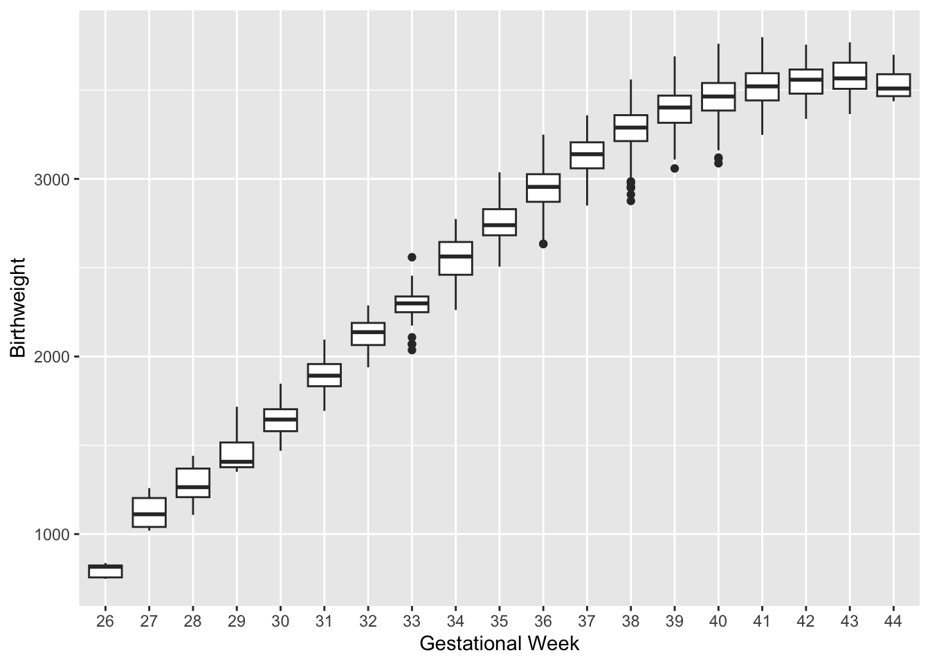
Motivating Example: Birthweight and Mothers Age In a 2023 study of low birth weight among infants in Georgia, data were collected for \(N = 5{,}000\) infants. Gestational age (in weeks) and maternal age were recorded to assess the relationship between gestational age and infant birthweight (in grams). The dataset includes the following variables:

• \(gw\) : gestational age in weeks.

• \(age\): maternal age at delivery

• \(bw\) birthweight at delivery in grams

• We see a non-linear relationship between \(gw\) and \(bw\) of a newborn.

---

Why Not linear regression? The wrong approach

Let’s fit a linear regression model as a baseline to assess how well it captures this relationship. We’ll then compare it to more flexible approaches, such as basis expansions or splines, to see if they provide a better fit.

Call:
lm(formula = bw ~ gw, data = dat)

Residuals:
    Min      1Q  Median      3Q     Max 
-761.50  -83.01   16.80  100.80  348.80 

Coefficients:
             Estimate Std. Error t value Pr(>|t|)    
(Intercept) -2177.513     39.351  -55.34   <2e-16 ***
gw            141.808      1.019  139.10   <2e-16 ***
---
Signif. codes:  0 '***' 0.001 '**' 0.01 '*' 0.05 '.' 0.1 ' ' 1

Residual standard error: 144.2 on 4998 degrees of freedom
Multiple R-squared:  0.7947,    Adjusted R-squared:  0.7947 
F-statistic: 1.935e+04 on 1 and 4998 DF,  p-value: < 2.2e-16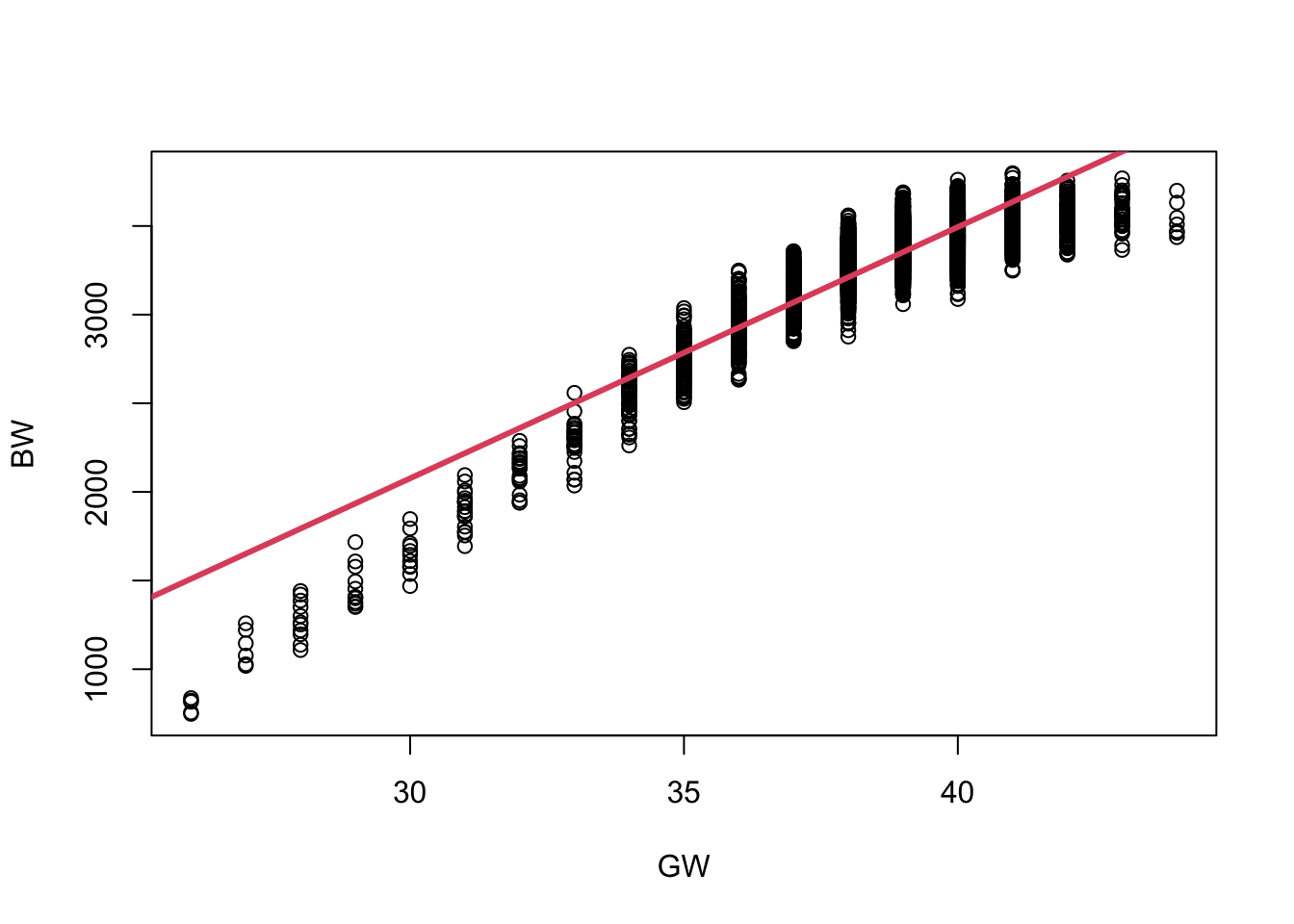

• The linear fit does not capture the non-linear trend in the relationship between gestational age (\(gw\)) and birthweight (\(bw\)).

• Overestimates birthweight at lower and higher gestational ages.

• Doesn’t capture curvature in the true relationship.

• Suggests the need for a more flexible modeling approach, such as basis expansions or splines, to better capture the underlying structure.

---

A Better Approach: Basis Expansions and Splines

Basis Expansion

• Consider the regression model:

\[ y_i = g(x_i) + \epsilon_i, \]

where \(g(x_i)\) represents the true, possibly non-linear relationship between the predictor \(x_i\) and the response \(y_i\), and \(\epsilon_i\) is the error term.

• One common approach is to express \(g(x_i)\) as a linear combination of \(M\) known basis functions \(b_m(x_i)\):

\[ g(x_i) = \sum_{m=1}^M \beta_m b_m(x_i), \]

where \(\beta_m\) are unknown coefficients to be estimated.

• \(b_m(x_i)\) are called Basis Function and are chosen and fixed a priori, serving as known transformations of the original predictor \(x_i\).

• Our task is to estimate the coefficients \(\beta_m\) corresponding to these transformed variables.

• Basis functions provide a flexible framework to model complex, non-linear relationships by representing \(g(x)\) as a combination of simpler functions. They are fundamental tools in functional data analysis and optimization, enabling the modeling of curves as piecewise or smoothly varying functions.

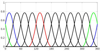
Below are some common examples of Basis Functions:

1. Polynomial Basis

Definition: A polynomial basis uses powers of the predictor variable to model non-linear trends. The basis functions are:

\[ b_1(x) = 1,\quad b_2(x) = x,\quad b_3(x) = x^2,\quad \ldots,\quad b_M(x) = x^{M-1} \]

Model:

\[ g(x) = \beta_0 + \beta_1 x + \beta_2 x^2 + \cdots + \beta_{M-1} x^{M-1} \]

Use Case: Polynomial bases are useful when the underlying relationship is smooth and continuous, such as quadratic or cubic trends. However, high-degree polynomials can lead to overfitting and numerical instability, especially near the boundaries (Runge’s phenomenon).

2. Indicator Basis (Step Functions)

Definition: An indicator basis partitions the domain of ( x ) into intervals and defines a separate basis function for each interval:

\[ b_m(x) = \begin{cases} 1 & \text{if } x \in I_m \\ 0 & \text{otherwise} \end{cases} \]

where ( I_m ) is the ( m^ ) interval.

Model:

\[ g(x) = \sum_{m=1}^M \beta_m \cdot \mathbb{1}_{\{x \in I_m\}} \]

Use Case: This approach is useful for piecewise constant modeling, especially when the data exhibit abrupt changes or discontinuities. However, the resulting model is not smooth, and predictions can jump sharply at the boundaries between intervals.

3. Periodic Basis (Fourier Series)

Definition: Periodic bases use sine and cosine functions to capture repeating patterns in the data. A typical Fourier basis includes terms like:

\[ b_1(x) = \sin(2\pi x),\quad b_2(x) = \cos(2\pi x),\quad b_3(x) = \sin(4\pi x),\quad \ldots \]

Model:

\[ g(x) = \beta_1 \sin(2\pi x) + \beta_2 \cos(2\pi x) + \cdots \]

Use Case: Periodic bases are ideal for cyclical data, such as seasonal trends (e.g., monthly temperatures, daily traffic volume). They provide a smooth, continuous fit and naturally model data that repeat over a fixed period.

Summary Table of Basis Function Types

Basis Type	Captures	Smoothness	Use Case
Polynomial	Global smooth trends	Smooth	Curved but continuous relationships
Indicator	Piecewise constant	Discontinuous	Sharp jumps or categorization
Periodic	Cyclical/repeating trends	Smooth	Seasonal or periodic data

---

Polynomial Regression

Let’s fit a Polynomial Regression to the birthweight outcomes:

\[ \begin{align*} \text{Quadratic } y_i & = \beta_0 + \beta_1 x_i + \beta_2 x_i^2 + e_i\\ \text{Cubic } y_i & = \beta_0 + \beta_1 x_i + \beta_2 x_i^2 + + \beta_3 x_i^3 + e_i\\ \end{align*} \]

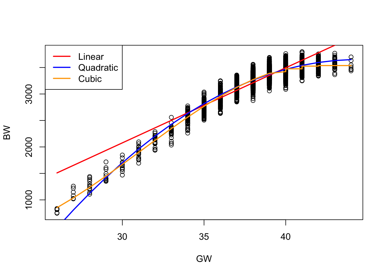
The linear model provides a general upward trend, but it fails to capture subtle curvature in the data, particularly at the extremes of gestational age. The quadratic model improves the fit by introducing curvature, better capturing the accelerating increase in birthweight with gestational age. However, it tends to oversimplify the relationship near the boundaries. The cubic model offers the most flexible fit among the three, capturing inflection points and more nuanced trends in the data. While it improves predictive accuracy, especially in the mid-gestational range, it also may introduce slight overfitting near the edges. Overall, higher-degree polynomials offer more flexibility but must be used cautiously to avoid instability and overfitting, particularly with extrapolation.

Note that all polynomial functions often cannot model the ends very well.

---

Fitting a Polynomial Regression in R

#Quadratic polynomial model
fit2 <- lm(bw ~ gw + I(gw^2), data = dat)

#Cubic polynomial model
fit3 <- lm(bw ~ gw + I(gw^2) + I(gw^3), data = dat)

Metric	Quadratic Model (fit2)	Cubic Model (fit3)
Model formula	\[ bw \sim gw + gw^2 \]	\[ bw \sim gw + gw^2 + gw^3 \]
Residual standard error	113.8	110.1
Adjusted ( R^2 )	0.872	0.880
F-statistic	17,030 (p < 2.2e-16)	12,240 (p < 2.2e-16)
Coefficient significance	All terms highly significant (p < 2e-16)	All terms highly significant (p < 2e-16)
Max residual	451.45	300.81
Interpretation of coefficients	Negative quadratic term indicates decreasing marginal effect of gestational weeks on birthweight	Cubic term allows more flexible curvature capturing subtle inflections

• Both quadratic and cubic models explain a large proportion of variance in birthweight, with adjusted \(R^2\) above 0.87.

• The cubic model shows a modest improvement over quadratic:

  • Lower residual standard error (110.1 vs 113.8)
  • Slightly higher adjusted \(R^2\) (0.880 vs 0.872)
  • Smaller maximum residuals (300.81 vs 451.45)

• All polynomial terms are highly statistically significant, confirming nonlinear relationships between gestational age and birthweight.

• The cubic term adds flexibility, capturing subtle curvature and inflection points missed by the quadratic model.

• However, the improvement is modest and higher-degree polynomials risk overfitting.

---

Piecewise Regression

One intuitive approach to modeling non-linear relationships between a predictor and the response is to divide the range of the predictor into several meaningful subregions. For example, consider pregnancy length as a predictor:

• Preterm: less than 37 weeks
  
• Full-term: 37 to 41 weeks
  
• Post-term: more than 42 weeks

Rather than fitting a single global polynomial across the entire range, we can model the relationship using polynomial functions separately within each region. This technique allows for greater flexibility and can better capture local patterns in the data without overfitting globally.

The values that define the boundaries between these regions—such as 37 and 42 weeks in the example above—are called knots.

Knots are central to methods such as piecewise regression, where the domain of the predictor is split at these points, and separate (yet smoothly connected) polynomial functions are fit in each subregion. This structure enables models to adapt to changes in the shape of the data while preserving continuity and smoothness.

Piecewise regression can be interpreted as a model in which the basis functions of \(x_i\) are allowed to interact with indicator (dummy) variables that define distinct regions of the predictor’s domain. For example:

where

\[ D_{1i} = \begin{cases} 1 & 37 \leq x_i < 42\\ 0 & OW \end{cases} \]

\[ D_{2i} = \begin{cases} 1 & x_i \geq 42\\ 0 & OW \end{cases} \]

We have two cut-points (knots) which yields three regions. We only need two dummy variables for three regions.

The piecewise quadratic regression model is expressed as:

\[ \begin{aligned} y_i =\ & \beta_0 + \beta_1 x_i + \beta_2 x_i^2 & \text{(Preterm baseline)} \\ & + \beta_3 D_{1i} + \beta_4 x_i D_{1i} + \beta_5 x_i^2 D_{1i} & \text{(Full-term adjustment)} \\ & + \beta_6 D_{2i} + \beta_7 x_i D_{2i} + \beta_8 x_i^2 D_{2i} & \text{(Post-term adjustment)} \end{aligned} \]

---

Fitting Piecewise Polynomial Regression Models in R

In this section, we demonstrate how to fit piecewise polynomial regression models by dividing the predictor variable — gestational weeks (\(gw\)) — into meaningful regions defined above and fitting separate polynomial models within each region. We use indicator variables for the regions and interact them with polynomial terms of \(gw\).

We divide the gestational weeks into three regions based on clinical definitions:

• Preterm: \(gw < 37\) weeks
  
• Full-term: \(37 \leq gw \leq 41\) weeks
  
• Post-term: \(gw \geq 42\) weeks

In R, we create logical vectors to indicate these regions:

The preterm region is implicitly defined where both Ind1 and Ind2 are FALSE.

We fit a linear model where the slope and intercept can differ by region through interaction terms:

fit4 = lm (bw~gw*(Ind1+ Ind2), data = dat)

#the syntax I(gw^2) can be used to calculate gw^2 within lm:
# also note use of parentheses to enumerate all terms

summary(fit4)

Call:
lm(formula = bw ~ gw * (Ind1 + Ind2), data = dat)

Residuals:
    Min      1Q  Median      3Q     Max 
-396.28  -74.28    4.34   78.34  321.34 

Coefficients:
             Estimate Std. Error t value Pr(>|t|)    
(Intercept) -4634.537     74.286  -62.39   <2e-16 ***
gw            210.735      2.158   97.67   <2e-16 ***
Ind1TRUE     4244.229     94.153   45.08   <2e-16 ***
Ind2TRUE     7710.241    711.475   10.84   <2e-16 ***
gw:Ind1TRUE  -114.351      2.620  -43.65   <2e-16 ***
gw:Ind2TRUE  -199.521     16.853  -11.84   <2e-16 ***
---
Signif. codes:  0 '***' 0.001 '**' 0.01 '*' 0.05 '.' 0.1 ' ' 1

Residual standard error: 111.8 on 4994 degrees of freedom
Multiple R-squared:  0.8766,    Adjusted R-squared:  0.8764 
F-statistic:  7092 on 5 and 4994 DF,  p-value: < 2.2e-16

Here, \(gw * (Ind1 + Ind2)\) expands to include:

• The main effect of \(gw\) (\(\beta_1\)): This represents the baseline linear effect of gestational week on birthweight in the preterm region (\(gw < 37\)). For each additional week, birthweight changes by \(\beta_1\) grams.

• The main effects of \(Ind_1\) and \(Ind_2\) (\(\beta_2\), \(\beta_3\)): These capture shifts in the intercept for the full-term and post-term regions, respectively, relative to the preterm baseline. In other words, they reflect differences in baseline birthweight at \(gw=0\) (hypothetical) between regions.

Interaction terms between \(gw\) and indicators:

• \(gw : Ind_1\) (Estimate = 1202, significant): The slope of \(gw\) in the full-term region is 1202 grams per week higher than in the preterm region. This means birthweight increases more steeply with gestational weeks in the full-term window.

• \(gw : Ind_2\) (Estimate = 2488, not significant): Suggests a higher slope in the post-term region, but this is not statistically significant, so no strong evidence the slope differs from preterm here.

Interaction terms between \(gw^2\) and indicators:

• \(gw^2 : Ind_1\) (Estimate = -16.85, significant): Indicates that the quadratic curvature in the full-term region bends downward more sharply compared to the preterm region, capturing a deceleration in growth.

• \(gw^2 : Ind_2\) (Estimate = -31.34, partial): Suggests similar curvature change in the post-term region, though significance would need to be checked.

• This model includes only linear terms for gw and allows both the intercept and the slope of gw to vary across the gestational age regions defined by Ind1 and Ind2.

More Flexible Model Specification

To model non-linear relationships between birthweight (bw) and gestational weeks (gw) that may vary across different gestational age regions (e.g., preterm, full-term, post-term), we may extend the model to include quadratic terms for gw.

The piecewise quadratic regression model with interaction terms can be written as:

\[ bw_i = \beta_0 + \beta_1 gw_i + \beta_2 gw_i^2 + \beta_3 Ind1_i + \beta_4 Ind2_i + \beta_5 (gw_i \times Ind1_i) + \beta_6 (gw_i \times Ind2_i) + \beta_7 (gw_i^2 \times Ind1_i) + \beta_8 (gw_i^2 \times Ind2_i) + \epsilon_i \]

This model allows both the intercept and the linear and quadratic effects of gestational weeks to vary across the three gestational age regions. This flexibility enables better modeling of complex, region-specific relationships between gestational age and birthweight.

fit5 = lm (bw~(gw + I(gw^2))*(Ind1+ Ind2), data = dat)

###Important
# In R formulas, the caret symbol (^) is not interpreted as exponentiation but as a formula operator indicating interactions or polynomial expansions of terms.
# 
# Writing (gw^2) without wrapping it in the I() function causes R to treat it as "gw to the power of 2" in the formula sense (interactions), not as the squared variable $gw^2$.
# 
# This leads to an unintended model structure that does not include the quadratic term properly, and may result in errors or nonsensical coefficients.
dontdothis = lm(bw~(gw+(gw^2))*(Ind1+ Ind2), data = dat)

fit6 = lm (bw~(gw+I(gw^2) + I(gw^3))*(Ind1+ Ind2), data = dat)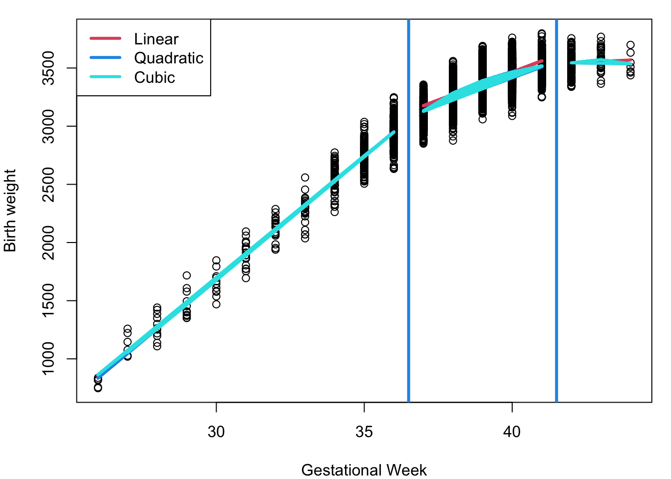

Limitations in Piecewise Polynomials:

• Limited flexibility in capturing complex trends: Although polynomial fits (linear, quadratic, cubic) are applied separately in each region, they often produce similar shapes, which may fail to represent subtle changes in the relationship between gestational age and birthweight—especially where the effect weakens at higher gestational weeks.

• Lack of smoothness at knots: The fitted curves generally do not join smoothly at the boundaries (knots) between regions. This can cause abrupt changes or discontinuities in the predicted values or their slopes, which is unrealistic for most natural processes.

• High model complexity: Fitting separate polynomials for each region requires estimating many parameters, increasing the degrees of freedom and the potential for overfitting, particularly with limited data.

---

Discontinuities at the Boundaries

Piecewise polynomial regression fits separate polynomial models within different intervals of the predictor variable separated by knots. While this allows for flexible modeling of nonlinear relationships, an important drawback is the potential for discontinuities at these knot points.

What is a discontinuity? A discontinuity occurs when the fitted function or its derivatives have abrupt changes at the knot locations. For example, suppose the predictor \(x\) is divided into two regions by a knot at \(k\). We fit two separate polynomial functions:

\[ g_1(x) = \beta_0^{(1)} + \beta_1^{(1)} x + \beta_2^{(1)} x^2, \quad x < k \]

\[ g_2(x) = \beta_0^{(2)} + \beta_1^{(2)} x + \beta_2^{(2)} x^2, \quad x \geq k \]

If these functions are not constrained to be equal at \(x = k\), then the value of \(g_1(k)\) may differ from \(g_2(k)\), causing a jump in the predicted curve.

1. Discontinuity in the function: If \(g_1(k) \neq g_2(k)\), the function is discontinuous at \(k\). This means the predicted response suddenly changes as we cross the knot, which is usually unrealistic for continuous processes like birthweight increasing with gestational age.
2. Discontinuity in derivatives: Even if \(g_1(k) = g_2(k)\), the slope or curvature may still jump,e.g.,

• If \(g_1'(k) \neq g_2'(k)\), the first derivative (slope) is discontinuous.

• If \(g_1''(k) \neq g_2''(k)\), the second derivative (curvature) is discontinuous.

Discontinuities in derivatives make the fitted curve look “kinked” or less smooth at the knots.

Why does this matter? Discontinuities reduce the smoothness of the regression curve. For biological or physical processes, smooth transitions are often expected.Piecewise polynomial regression without additional constraints does not guarantee continuity or smoothness at the knots.

---

Summary

Section	Description
What is the Model?	A basis expansion model expresses an unknown function \(g(x)\) as a linear combination of known basis functions: \(g(x_i) = \sum_{m=1}^M \beta_m b_m(x_i)\) The goal is to flexibly model nonlinear relationships by choosing appropriate basis functions \(b_m(\cdot)\).
Polynomial Basis	Uses powers of \(x\) as basis functions: \(b_1(x) = 1, \quad b_2(x) = x, \quad b_3(x) = x^2, \quad \ldots, \quad b_M(x) = x^{M-1}\) Leads to polynomial regression models like quadratic or cubic regression.
Piecewise Polynomial Basis	Divides the domain of \(x\) into intervals with knots and fits separate polynomials on each interval. Uses indicator functions \(D_i\) to select intervals, e.g., \(y_i = \beta_0 + \beta_1 x_i + \beta_2 x_i^2 + \beta_3 D_{1i} + \beta_4 x_i D_{1i} + \ldots\)
Indicator Variables (Knots)	\(D_{1i}, D_{2i}, \ldots\) are defined to indicate which interval \(x_i\) belongs to, enabling piecewise definitions of the function. E.g., \(D_{1i} = 1\) if \(x_i\) in interval 1, else 0. Allows flexibility but can cause discontinuities at knots if not constrained.
Parametric Splines	Piecewise polynomials with constraints (e.g., continuity, smoothness) at knots to avoid jumps or sharp corners. Ensures the function and its derivatives match at knots, yielding smooth curves useful in regression and smoothing applications.
Why Use Basis Expansions?	To model nonlinear effects in regression flexibly while retaining a linear structure in parameters \(\beta_m\), enabling standard estimation methods like least squares. Basis expansions allow balancing flexibility and interpretability.
Key R Modeling Note	In R formulas, polynomial terms like \(x^2\) must be wrapped in I() to indicate arithmetic, e.g., I(x^2), otherwise caret ^ is interpreted as formula syntax (e.g., interaction).
Continuity and Smoothness	Without constraints, piecewise polynomials can be discontinuous or have sharp corners at knots. Parametric splines enforce conditions so that the function is continuous and smooth (derivatives continuous) across knots, improving fit quality and interpretability.