4.2 Time Domain TSA

• Prophet
  • Prophet is a procedure for forecasting time series data based on an additive model where non-linear trends are fit with yearly, weekly, and daily seasonality, plus holiday effects. It works best with time series that have strong seasonal effects and several seasons of historical data.
  • Prophet is robust to missing data and shifts in the trend, and typically handles outliers well.
• Forecasting: Principles and Practice, V3
• Machine Learning with R, the tidyverse, and mlr
• Some R Time Series Issues, TSA2

4.2.1 tsibbles, feasts, fable

• Time series graphics using feasts
• Tidy time series data using tsibbles
• Electricity demand data in tsibble format
• Reintroducing tsibble: data tools that melt the clock

The fable ARIMA() function uses an alternate parameterisation of constants to stats::arima() and forecast::Arima(). While the parameterisations are equivalent, the coefficients for the constant/mean will differ.

In fable, the parameterisation used is:

\[ (1-φ_1B - \cdots - φ_p B^p)(1-B)^d y_t = c + (1 + θ_1 B + \cdots + θ_q B^q)\varepsilon_t \]

In stats and forecast, an ARIMA model is parameterised as:

\[ (1-φ_1B - \cdots - φ_p B^p)(y_t' - μ) = (1 + θ_1 B + \cdots + θ_q B^q)\varepsilon_t \]

where μ is the mean of \((1-B)^d y_t\) and \(c = μ(1-φ_1 - \cdots - φ_p)\).

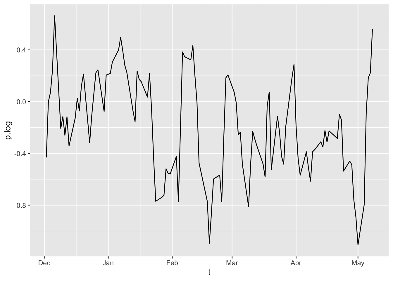
4.2.2 Interpretation

4.2.3 Autoregressions (AR)

For example 4.1, it can be visualised:

When using other functions in feasts, the univaraite time series must be specified.

tsi_fulton %>% feasts::gg_tsdisplay(p.log)

tsi_fulton %>% ACF(p.log) %>% autoplot()

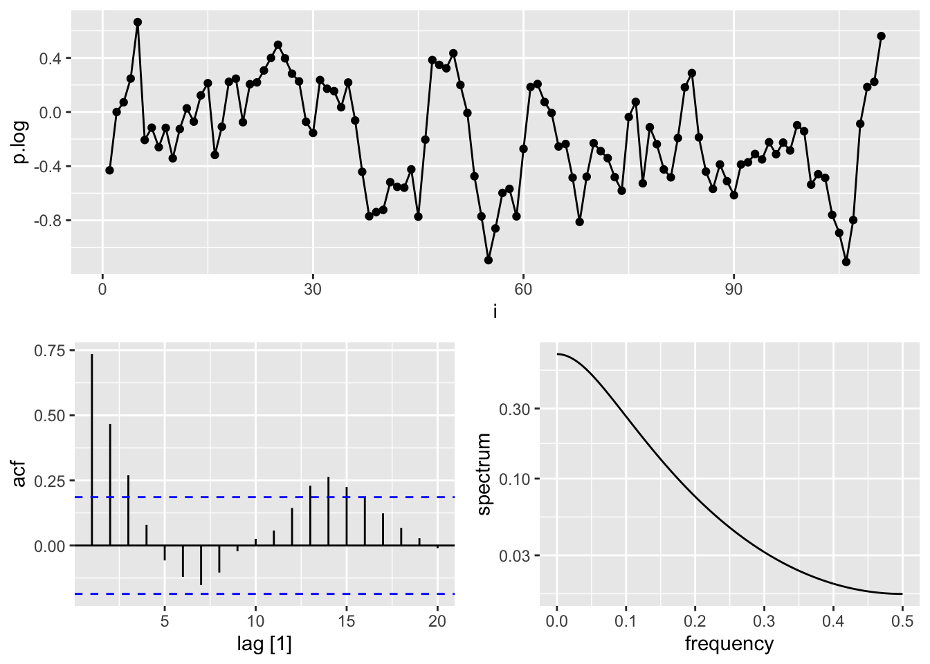
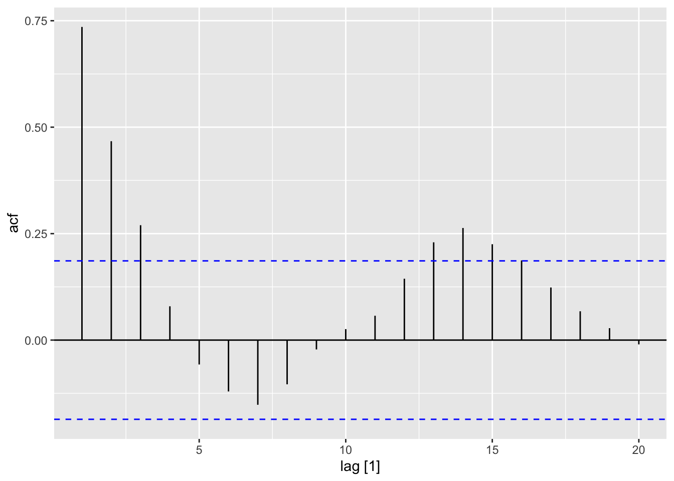
4.2.3.1 Models

mods_fulton[[1]] %>% glance() %>% tab_ti()

.model	sigma2	log_lik	AIC	AICc	BIC	ar_roots	ma_roots
fable::ARIMA(p.log ~ 1 + pdq(1, 0, 0))	0.06436	-4.67	15.34	15.56	23.47	1.31917441155036+0i	complex(0)

mods_fulton[[1]] %>% tidy() %>% tab_ti()

.model	term	estimate	std.error	statistic	p.value
fable::ARIMA(p.log ~ 1 + pdq(1, 0, 0))	ar1	0.75805	0.06287	12.058	6.601e-22
fable::ARIMA(p.log ~ 1 + pdq(1, 0, 0))	constant	-0.04351	0.02324	-1.872	6.379e-02

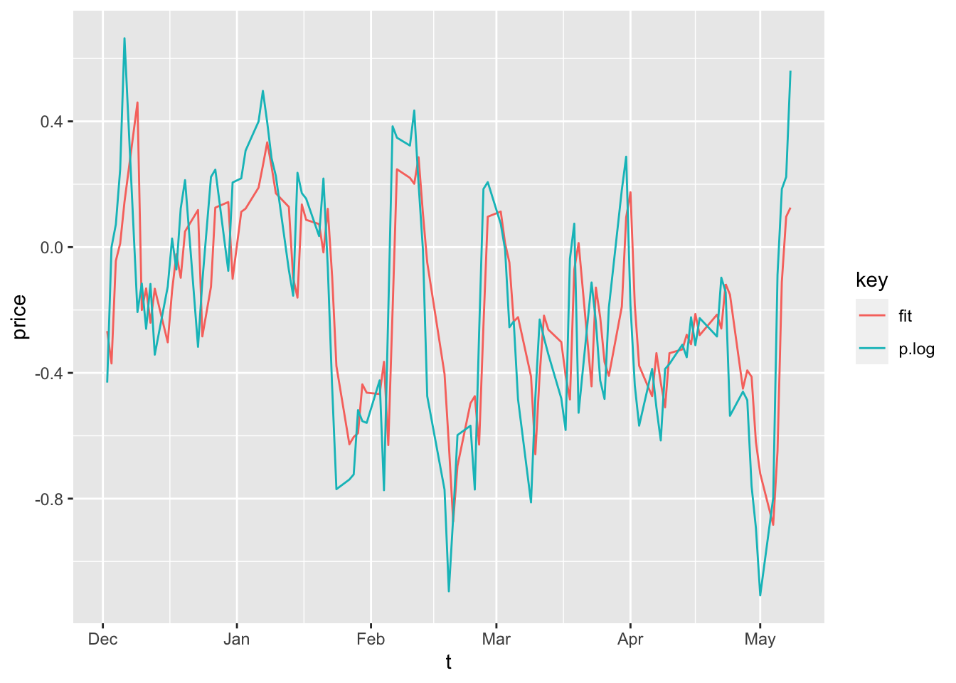
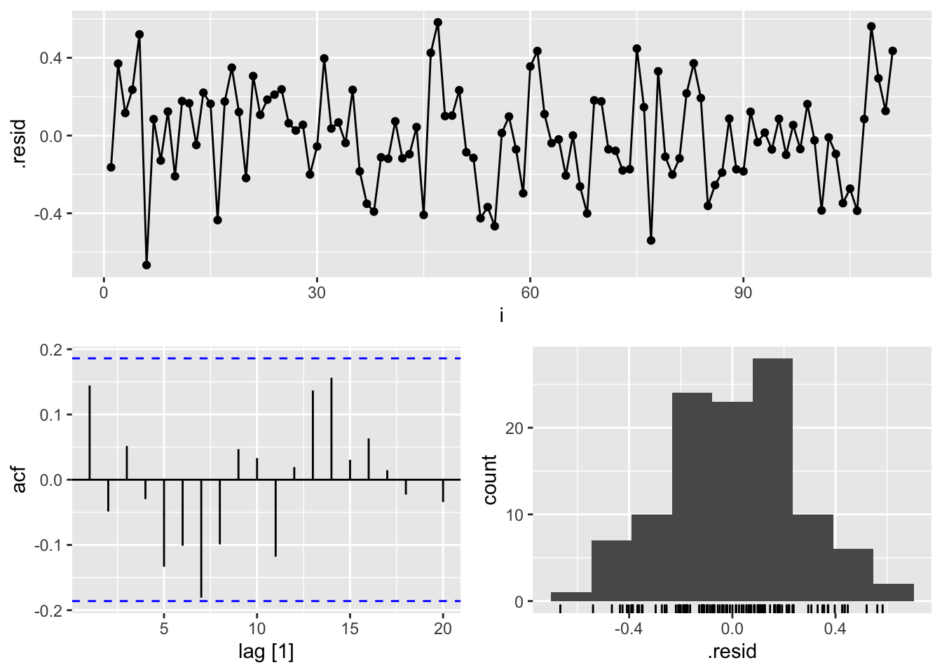
The model residuals can be analysed using function gg_tsresiduals().

and function qqPlot().

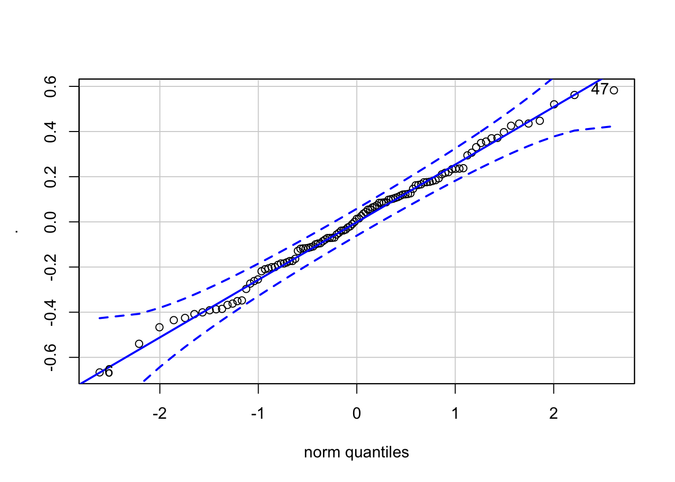
#> [1]  6 47

4.2.4 Inference

Log Likelihood Ratio Test

whi	stat	df1	df2	p_value	prob	if_reject
logLik	90.98	1	110	0	0.05	TRUE

4.2.5 Mis-Specification Analysis (MSA)

mods_fulton[[1]] %>% test_jb_tsi() %>% tab_ti()

#> Registered S3 method overwritten by 'propagate':
#>   method         from   
#>   print.interval tsibble

whi	stat	df1	df2	p_value	prob	if_reject
Jarque-Bera	0.3879	2	109	0.8237	0.05	FALSE

mods_fulton[[1]] %>%
  residuals() %>%
  features(.resid, ljung_box) %>%
  tab_ti()

.model	lb_stat	lb_pvalue
fable::ARIMA(p.log ~ 1 + pdq(1, 0, 0))	2.381	0.1228