2.3 Interval Estimation
2.3.1 Confidence Interval of Parameters
The width of these confidence intervals is a measure of the overall quality of the regression line. (Montgomery, Peck, and Vining 2012)
By choosing a 95% coverage, we accept that with 5% confidence we reach the false conclusion that the true parameter is not in the confidence interval. – section 2.3.1 confidence intervals in (Hendry and Nielsen 2007)
For example, the confidence interval of mods_recs[[1]] can be calculated using stats::confint().
| 2.5 % | 97.5 % |
|---|---|
| 8.220362 | 9.010864 |
| -0.317329 | -0.202613 |
| -0.156244 | -0.006692 |
| 0.026693 | 0.102253 |
| -0.176156 | 0.107756 |
| 0.002521 | 0.011981 |
| -0.021882 | 0.048176 |
2.3.2 Confidence Interval of Mean Responses
A major use of a regression model is to estimate the mean response \(\mathrm{E}(y)\) for a particular value of the regressor variable \(x\). (Montgomery, Peck, and Vining 2012)
2.3.3 Prediction Interval of New Observations
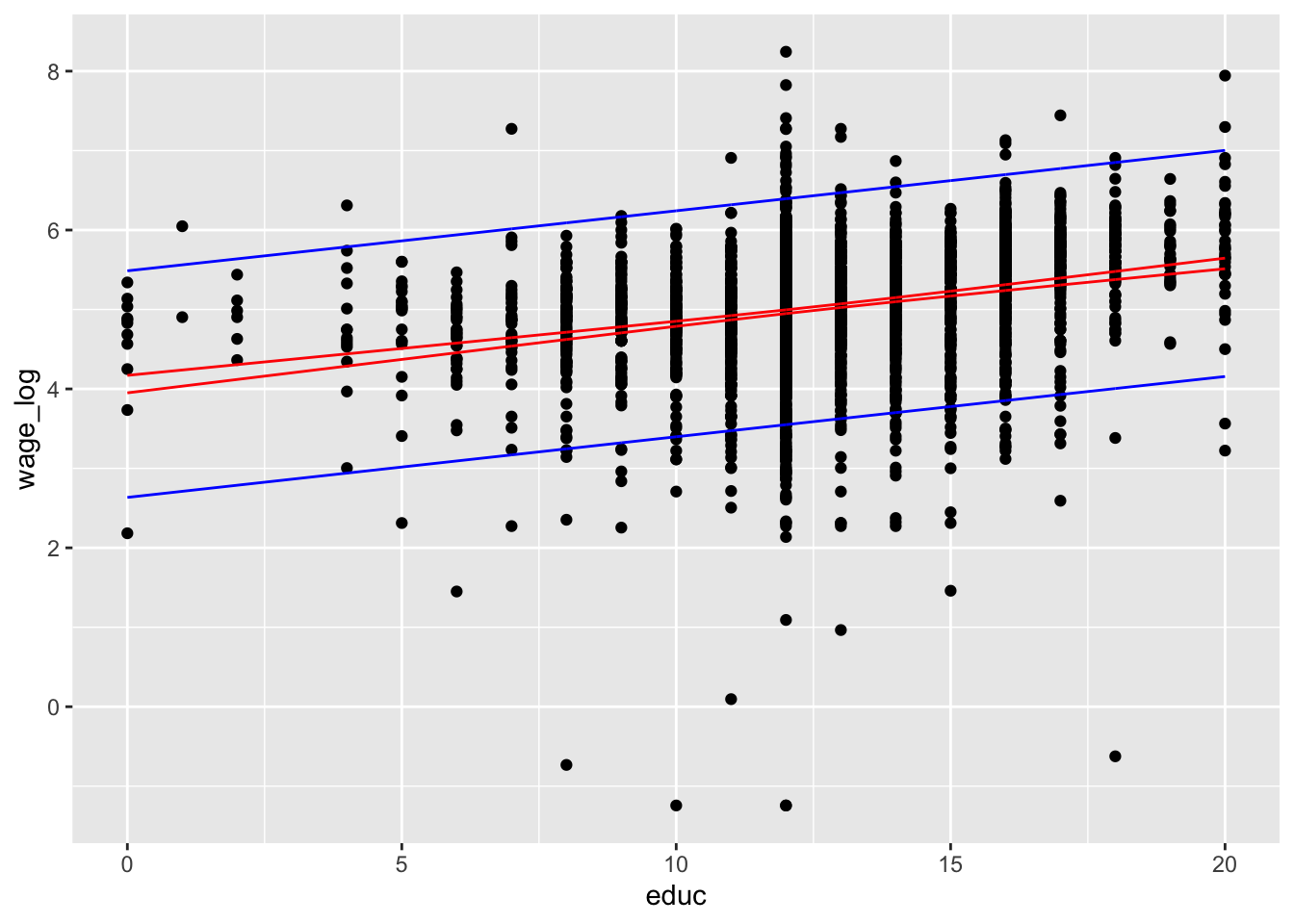
The CI on the mean response is inappropriate for this problem because it is an interval estimate on the mean of y (a parameter), not a probability statement about future observations from that distribution. (Montgomery, Peck, and Vining 2012)
int_pred <-
  mods_census[[1]] %>%
  predict(newdata = data.frame(educ = dat_census$educ),
    interval = "prediction", level = .95) %>%
  as_tibble() %>%
  select(lwr.pred = lwr, upr.pred = upr)
add_predictions() can be used to generate predictions.
| educ | wage_log | pred |
|---|---|---|
| 15 | 5.260 | 5.200 |
| 16 | 3.223 | 5.276 |
| 14 | 5.212 | 5.124 |
| 12 | 5.373 | 4.972 |
| 12 | 6.927 | 4.972 |
References
Hendry, David F, and Bent Nielsen. 2007. Econometric Modeling: A Likelihood Approach. Princeton University Press.
Montgomery, Douglas C, Elizabeth A Peck, and G Geoffrey Vining. 2012. Introduction to Linear Regression Analysis. Vol. 821. John Wiley & Sons.