2.2 Multiple Linear Regression
2.2.1 Standardisation
2.2.2 Multicollinearity Diagnosis
In some situations the regressors are nearly perfectly linearly related, and in such cases the inferences based on the regression model can be misleading or erroneous. When there are near-linear dependencies among the regressors, the problem of multicollinearity is said to exist. – chapter 9 in (Montgomery, Peck, and Vining 2012)
There are four primary sources of multicollinearity: – chapter 9 in (Montgomery, Peck, and Vining 2012)
- The data collection method employed
- Constraints on the model or in the population
- Model specification
- An overdefined model
To really establish causation, it is usually necessary to do an experiment in which the putative causative variable is manipulated to see what effect it has on the response. – section 1.5.7 in (Wood 2017 :)
(1) Covariance Matrix
Inspection of the covariance matrix is not sufficient for detecting anything more complex than pair- wise multicollinearity. – section 9.4.1 Examination of the Correlation Matrix in (Montgomery, Peck, and Vining 2012)
For example, it can be seen from the following covariance matrix that y is highly correlated to x2, x6 and x8. Besides, x3-x4, x2-x6, x4-x8 are high correlated.
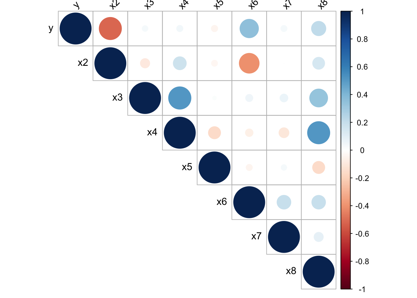
Figure 2.1: Heat map for the covariance matrix of recs.
(2) Variance Inflation Factors (VIF)
The collinearity diagnostics in R require the packages “perturb” and “car”. The R code to generate the collinearity diagnostics for the delivery data is:
#>     case     dist
#> 3.118474 3.118474
#> Condition
#> Index Variance Decomposition Proportions
#> intercept case dist
#> 1 1.000 0.041 0.015 0.016
#> 2 3.240 0.959 0.069 0.076
#> 3 6.378 0.000 0.915 0.909#> x2 x3 x4 x5 x6 x7
#> 1.303049 1.477179 1.555868 1.041024 1.264788 1.085367#> Condition
#> Index Variance Decomposition Proportions
#> intercept x2 x3 x4 x5 x6 x7
#> 1 1.000 0.001 0.004 0.002 0.004 0.008 0.002 0.006
#> 2 3.355 0.000 0.009 0.003 0.051 0.762 0.000 0.000
#> 3 4.236 0.000 0.035 0.003 0.129 0.098 0.014 0.464
#> 4 4.817 0.000 0.520 0.034 0.062 0.002 0.024 0.018
#> 5 6.328 0.027 0.014 0.001 0.264 0.063 0.180 0.500
#> 6 9.107 0.001 0.003 0.774 0.479 0.038 0.153 0.011
#> 7 15.967 0.971 0.415 0.184 0.011 0.028 0.626 0.0012.2.3 Orthogonalisation
This will facilitate solving the likelihood equations, and also help the general interpretation and use of regression models. (Hendry and Nielsen 2007)
Orthogonalizing the regressors does not change the model and the likelihood, but it eliminates the near collinearity. (Hendry and Nielsen 2007)
In contrast to this situation, perfect collinearity is unique to the model and cannot be eliminated by orthogonalization. (Hendry and Nielsen 2007)
For example, regressors in mods_recs[[4]] can be orthogonalised to have a better model mods_recs[[5]].
#> lm(formula = y ~ z1 + z2 + z3, data = .)| term | estimate | std.error | statistic | p.value |
|---|---|---|---|---|
| (Intercept) | 8.35989 | 0.03397 | 246.088 | 0.000e+00 |
| z1 | -0.26998 | 0.02454 | -11.002 | 7.830e-24 |
| z2 | 0.06962 | 0.01105 | 6.301 | 1.067e-09 |
| z3 | 0.03271 | 0.01248 | 2.621 | 9.217e-03 |
| r.squared | adj.r.squared | sigma | statistic | p.value | df | logLik | AIC | BIC | deviance | df.residual |
|---|---|---|---|---|---|---|---|---|---|---|
| 0.3616 | 0.3551 | 0.5884 | 55.88 | 1.196e-28 | 4 | -264.6 | 539.1 | 557.6 | 102.5 | 296 |
The intercept parameter would have a more reasonable interpretation in a reparametrized model. (Hendry and Nielsen 2007)
The intercept (8.36) in mods_recs[[5]] can be interpreted as the exptected value for an individual with average values of x2, x8 and I(x2^2), which can be verified by the prediction using mods_recs[[4]].
( 8.75527 - 0.51392 * mean(dat_recs$x2) + 0.07631 * mean(dat_recs$x8) +
  0.03271 * mean(dat_recs$x2^2) ) - 8.35989 <= 1e-4
#> [1] TRUESince the standard errors in mods_recs[[5]] are smaller than those in mods_recs[[4]], mods_recs[[5]] is used to conduct inference. Particularly, se for Intercept is reduced by 75.48%, and ses for first two regressors are reduced by 71.75% and 2.41%. The estimations for the last term are exactly the same, which is expected.
References
Hendry, David F, and Bent Nielsen. 2007. Econometric Modeling: A Likelihood Approach. Princeton University Press.
Montgomery, Douglas C, Elizabeth A Peck, and G Geoffrey Vining. 2012. Introduction to Linear Regression Analysis. Vol. 821. John Wiley & Sons.
Wood, Simon N. 2017. Generalized Additive Models: An Introduction with R. CRC press.